EP0166547A2 - Vehicle navigational apparatus - Google Patents
Vehicle navigational apparatus Download PDFInfo
- Publication number
- EP0166547A2 EP0166547A2 EP85303898A EP85303898A EP0166547A2 EP 0166547 A2 EP0166547 A2 EP 0166547A2 EP 85303898 A EP85303898 A EP 85303898A EP 85303898 A EP85303898 A EP 85303898A EP 0166547 A2 EP0166547 A2 EP 0166547A2
- Authority
- EP
- European Patent Office
- Prior art keywords
- vehicle
- probable
- current
- dead reckoned
- street
- Prior art date
- Legal status (The legal status is an assumption and is not a legal conclusion. Google has not performed a legal analysis and makes no representation as to the accuracy of the status listed.)
- Granted
Links
- 238000000034 method Methods 0.000 claims abstract description 27
- 230000004044 response Effects 0.000 claims abstract description 22
- 238000009825 accumulation Methods 0.000 claims description 12
- 230000008859 change Effects 0.000 claims description 12
- 230000001419 dependent effect Effects 0.000 claims description 10
- 230000000717 retained effect Effects 0.000 claims description 7
- 230000003247 decreasing effect Effects 0.000 claims description 6
- 230000033001 locomotion Effects 0.000 claims description 6
- 238000009826 distribution Methods 0.000 claims description 4
- 238000004422 calculation algorithm Methods 0.000 abstract description 30
- 238000012360 testing method Methods 0.000 description 36
- 238000005314 correlation function Methods 0.000 description 20
- 230000000875 corresponding effect Effects 0.000 description 19
- 238000004364 calculation method Methods 0.000 description 17
- 230000006870 function Effects 0.000 description 13
- 238000012937 correction Methods 0.000 description 8
- 230000004907 flux Effects 0.000 description 8
- 230000008569 process Effects 0.000 description 7
- 238000011156 evaluation Methods 0.000 description 6
- 238000005259 measurement Methods 0.000 description 6
- 238000004590 computer program Methods 0.000 description 4
- 238000010586 diagram Methods 0.000 description 4
- 238000012545 processing Methods 0.000 description 4
- 238000013459 approach Methods 0.000 description 3
- 238000012544 monitoring process Methods 0.000 description 3
- 238000001914 filtration Methods 0.000 description 2
- 230000009467 reduction Effects 0.000 description 2
- 240000006829 Ficus sundaica Species 0.000 description 1
- 229910000831 Steel Inorganic materials 0.000 description 1
- 230000001133 acceleration Effects 0.000 description 1
- 230000008901 benefit Effects 0.000 description 1
- 230000003139 buffering effect Effects 0.000 description 1
- 238000004891 communication Methods 0.000 description 1
- 230000002596 correlated effect Effects 0.000 description 1
- 238000013500 data storage Methods 0.000 description 1
- 230000000881 depressing effect Effects 0.000 description 1
- 238000009795 derivation Methods 0.000 description 1
- 238000001514 detection method Methods 0.000 description 1
- 230000008030 elimination Effects 0.000 description 1
- 238000003379 elimination reaction Methods 0.000 description 1
- 238000005516 engineering process Methods 0.000 description 1
- 238000007689 inspection Methods 0.000 description 1
- 238000012423 maintenance Methods 0.000 description 1
- 238000013077 scoring method Methods 0.000 description 1
- 239000010959 steel Substances 0.000 description 1
- 230000000007 visual effect Effects 0.000 description 1
Images


Classifications
-
- G—PHYSICS
- G06—COMPUTING; CALCULATING OR COUNTING
- G06F—ELECTRIC DIGITAL DATA PROCESSING
- G06F17/00—Digital computing or data processing equipment or methods, specially adapted for specific functions
-
- G—PHYSICS
- G09—EDUCATION; CRYPTOGRAPHY; DISPLAY; ADVERTISING; SEALS
- G09B—EDUCATIONAL OR DEMONSTRATION APPLIANCES; APPLIANCES FOR TEACHING, OR COMMUNICATING WITH, THE BLIND, DEAF OR MUTE; MODELS; PLANETARIA; GLOBES; MAPS; DIAGRAMS
- G09B29/00—Maps; Plans; Charts; Diagrams, e.g. route diagram
- G09B29/10—Map spot or coordinate position indicators; Map reading aids
- G09B29/106—Map spot or coordinate position indicators; Map reading aids using electronic means
-
- G—PHYSICS
- G01—MEASURING; TESTING
- G01C—MEASURING DISTANCES, LEVELS OR BEARINGS; SURVEYING; NAVIGATION; GYROSCOPIC INSTRUMENTS; PHOTOGRAMMETRY OR VIDEOGRAMMETRY
- G01C21/00—Navigation; Navigational instruments not provided for in groups G01C1/00 - G01C19/00
- G01C21/10—Navigation; Navigational instruments not provided for in groups G01C1/00 - G01C19/00 by using measurements of speed or acceleration
- G01C21/12—Navigation; Navigational instruments not provided for in groups G01C1/00 - G01C19/00 by using measurements of speed or acceleration executed aboard the object being navigated; Dead reckoning
- G01C21/14—Navigation; Navigational instruments not provided for in groups G01C1/00 - G01C19/00 by using measurements of speed or acceleration executed aboard the object being navigated; Dead reckoning by recording the course traversed by the object
-
- G—PHYSICS
- G01—MEASURING; TESTING
- G01C—MEASURING DISTANCES, LEVELS OR BEARINGS; SURVEYING; NAVIGATION; GYROSCOPIC INSTRUMENTS; PHOTOGRAMMETRY OR VIDEOGRAMMETRY
- G01C21/00—Navigation; Navigational instruments not provided for in groups G01C1/00 - G01C19/00
- G01C21/26—Navigation; Navigational instruments not provided for in groups G01C1/00 - G01C19/00 specially adapted for navigation in a road network
- G01C21/28—Navigation; Navigational instruments not provided for in groups G01C1/00 - G01C19/00 specially adapted for navigation in a road network with correlation of data from several navigational instruments
- G01C21/30—Map- or contour-matching
Definitions
- the present invention relates generally to an apparatus and method for providing information to improve the accuracy of tracking vehicles movable primarily over streets, as well as to an automatic vehicle navigational system and method for tracking the vehicles as they move over the streets.
- a variety of automatic vehicle navigational systems has been developed and used to provide information about the actual location of a vehicle as it moves over streets.
- a common purpose of the vehicle navigational systems is to maintain automatically knowledge of the actual location of the vehicle at all times as it traverses the streets (i.e., track the vehicle).
- a given navigational system may be utilized in the vehicle to provide the vehicle operator with knowledge of the location of the vehicle and/or at a central monitoring station that may monitor the location of one or more vehicles.
- dead reckoning in which the vehicle is tracked by advancing a “dead reckoned position” from measured distances and courses or headings.
- a system based upon dead reckoning principles may, for example, detect the distance traveled and heading of the vehicle using distance and heading sensors on the vehicle. These distance and heading data are then processed by, for example, a computer using known equations to calculate periodically a dead reckoned position DRP of the vehicle. As the vehicle moves along a street, an old dead reckoned position DRP is advanced to a new or current dead reckoned position DRP in response to the distance and heading data being provided by the sensors.
- the additional information may be a map corresponding to the streets of a given area over which the vehicle may be moving.
- the map is stored in memory as a map data base and is accessed by the computer to process this stored information in relation to the dead reckoned positions.
- U.S. Patent 3,789,198 discloses a vehicle location monitoring system using dead reckoning for tracking motor vehicles, including a technique for compensating for accumulated errors in the dead reckoned positions.
- a computer accesses a stored map data base, which is a table or array having a 2-dimensional orthogonal grid of entries of coordinates X st Y st that may or may not correspond to driveable surfaces, such as streets St. Storage locations in the array that correspond to streets are indicated by a logic 1, while all other storage locations are filled with a logic 0.
- a dead reckoned position DRP of the vehicle is periodically calculated, which position DRP is identified and temporarily stored in the computer as coordinates X old Yold. Then, to compensate for the accumulated error, the array is interrogated at a location corresponding to the coordinates X old Y old . If a logic 1 is found, the vehicle is defined as corresponding to a known driveable surface and no correction is made. If a logic 0 is found, representing no driveable surface, adjacent entries in the array are interrogated, as specifically described in the patent.
- Landfall is an acronym for Links And Nodes Database For Automatic Landvehicle Location, in which a stored map data base comprises roads (links) that are interconnected by junctions (nodes) having inlet/outlet ports.
- links links
- nodes junctions
- any mapped area is regarded merely as a network of nodes, each containing a number of inlet/outlet ports, and interconnected links.
- the publication describes the basic vehicle navigational algorithm used under the Landfall principle by assuming that a vehicle is on a road or link moving towards a node which it will enter by an input port. As the vehicle moves forward, the motion is detected by a distance encoder and the "distance-to-go", i.e., the distance to go to the next node, is decremented until it becomes zero, corresponding to the entry point of the input port of such a node. Then, as the vehicle exits one of several output ports of the node, a change of heading of the vehicle at the exit point with respect to the entry point is measured.
- the map data base for that node is scanned for an exit port matching the measured change in heading and, once identified, this exit port leads to the entry point of another node and the distance-to-go to that other node. Landfall attempts to compensate for the accumulation of error resulting from the achievable accuracy of the distance encoder by cancelling the error when the vehicle encounters a node and turns onto an exit port. More details of this vehicle navigational algorithm are disclosed in the publication.
- a common problem with the above-mentioned systems is the use of limited information to compensate for the accumulation of error, so as to accurately track a vehicle.
- this limited information is a coarse and simplistic representation of streets by logic 1 and logic 0 data of the map data base.
- Landfall system a relatively simplistic assumption is made that vehicles are always on a street of the map.
- the vehicle navigational algorithms of the patent and Landfall do not develop an estimate of correct location accuracy and use this information in dependence with the map data base to determine if the vehicle is on a street or not. Systems that do not maintain this estimate are more likely to update the position incorrectly or to fail to update the position when it should be.
- an apparatus for providing information to improve the accuracy of tracking a vehicle movable over streets in a given area including first means for providing data identifying respective positions of the vehicle, each position having an accuracy relative to an actual location of the vehicle and one of the positions being a current position, second means for providing a map data base of the streets, and means for deriving any of a plurality of parameters in dependence on one or more respective positions of the vehicle and the streets of the map data base to determine if a more probable current position exists.
- the invention is a method for providing information to improve the accuracy of tracking a vehicle movable over streets in a given area, including the steps of providing data identifying respective positions of the vehicle, each position having an accuracy relative to an actual location of the vehicle and one of the positions being a current position, providing a map data base of the streets, and deriving any of a plurality of parameters in dependence on one or more respective positions of the vehicle and the streets of the map data base to determine if a more probable current position exists.
- a significant amount of information in the form of the plurality of parameters may be derived from the positions of the vehicle and the map data base. Furthermore, and as will be described more fully below, this information may be used not necessarily to correct or update the current position of the vehicle, but at least to determine if a more probable current position exists.
- the present invention is an apparatus for automatically tracking a vehicle movable about streets of an overall given area, including first means for providing first data identifying respective positions of the vehicle as the vehicle moves about the streets, each position having a certain accuracy and one of the positions being a current position, second means for providing second data being an estimate of the accuracy of the respective positions of the vehicle, the estimate changing as the vehicle moves about the streets to reflect the accuracy of the respective positions, third means for providing a map data base of the streets of the given area, and means for determining if a more probable position than the current position exists in response to the first data, the second data and the map data base.
- the present invention is a method for automatically tracking a vehicle movable about streets of an overall given area including providing first data identifying respective positions of the vehicle as the vehicle moves about the streets, each position having a certain accuracy and one of the positions being a current position, providing second data being an estimate of the accuracy of the respective positions of the vehicle, the estimate changing as the vehicle moves about the streets to reflect the accuracy of the respective positions, providing a map data base of the streets of the given area, and determining if a more probable position than the current position exists in response to the first data, the second data and the map data base.
- the vehicle is tracked by determining if a more probable position than the current position exists. If a more probable current position is determined, then the current position is corrected (updated), but if a more probable position cannot be found, the current position is not updated. This determination is made in response to the data about the positions of the vehicle, the data which are an estimate of the accuracy of the respective positions of the vehicle and the map data base.
- the present invention will be discussed specifically in relation to automatic vehicle location systems using dead reckoning, which is one approach to tracking a vehicle movable over streets.
- the present invention may have application to other approaches to the problem of automatic vehicle location for tracking vehicles moving over streets, including, for example, "proximity detection" systems which use signposts that typically are, for example, low power radio transmitters located on streets to sense and transmit information identifying the location of a passing vehicle, as well as to Landfall-type systems previously described.
- the present invention also may have application in conjunction with yet other systems of providing information of the location of a vehicle movable over streets, such as land-based radio and/or satellite location systems.
- the vehicle that will be discussed may be a motor vehicle, such as a car, a recreational vehicle (RV), a motorcycle, a bus or other such type of vehicle primarily movable over streets.
- RV recreational vehicle
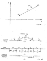
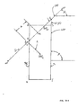
- Figs. 1A-1C are used to explain the basic principles of dead reckoning for tracking a moving vehicle V. Accordingly, Fig. 1A shows an XY coordinate system in which a vehicle V is moving over an actual street St from an arbitrary first or old location L at coordinates X Y to a new or current location L at coordinates X Y .
- an old dead reckoned position DRP has been calculated, as described below, which coincides with the actual location L of the vehicle 0 V, thereby also having coordinates X o Y o .
- a new or current dead reckoned position DRP is to be calculated when the vehicle V is at c its new or current location L .
- the old dead c reckoned position DRP o is advanced to the current dead reckoned position DRP by a calculation using well-known equations as follows: where X c Y c are the coordinates of DRP c , ⁇ D is a measured distance traveled by the vehicle V between L o and L , and H is a measured heading of the vehicle V.
- Fig. 1A assumes that there has been no error in calculating the current dead reckoned position DRP c . That is, the current dead reckoned position DRP c is shown to coincide exactly with the actual location L c of the vehicle V, whereby L and DRP have the identical coordinates X Y .
- FIG. 1B illustrates the more general situation in which errors are introduced into the calculation of the current dead reckoned position DRP c .
- the current dead reckoned position DRP will differ from the actual location L c of the vehicle V by an error E.
- This error E can arise due to a number of reasons. For example, the measurements of the distance ⁇ D and the heading H obtained with distance and heading sensors (not shown in Figs. 1A-1C) on the vehicle V may be inaccurate. Also, equations (1) and (2) are valid only if the vehicle V travels over distance ⁇ D at a constant heading H. Whenever the heading H is not constant, error is introduced into the calculation.
- the error E unless compensated, will on average accumulate as the vehicle V continues to move over the street St since X Y becomes X Y for each new calculation of the dead 0 0 reckoned position DRP in accordance with equations (1) and (2). This is indicated in Fig. 1B by showing the vehicle V at a subsequent new location L' c , together with a subsequent current dead reckoned position DRP' c and an accumulated error E' >E.
- any given DRP has a certain inaccuracy associated with it corresponding to the error E.
- Fig. 1C is used to explain generally the manner in which the error E associated with a given current dead reckoned position DRP c is compensated.
- Fig. 1C shows the vehicle V at location L , together with a current dead reckoned position DRP c and an error E, as similarly illustrated in Fig. 1B.
- a determination will be made if a more probable position than the current dead reckoned position DRP exists. If it is determined that a more probable position does exist, then the current dead reckoned position DRP is changed or updated to a certain XY coordinate corresponding to a point on the street St, identified as an updated current dead reckoned position DRP .
- the DRP may or may not coincide with the actual location L of the vehicle c (shown in Fig. 1C as not coinciding), but has been determined to be the most probable position at the time of updating. Alternatively, at this time it may be determined that no more probable position than the current dead reckoned position DRP c can be found, resulting in no changing or updating of the current dead reckoned position DRP. If the updating does occur, then the XY coordinates of the DRP cu become X o Y o in equations (1) and (2) for the next advance, whereas if no updating occurs at this time, then the XY coordinates of the DRP become X o Y o .
- Fig. 2 illustrates one embodiment of an automatic vehicle navigational system 10 of the present invention.
- a computer 12 accesses a data storage medium 14, such as a tape cassette or floppy or hard disk, which stores data and software for processing the data in accordance with a vehicle navigational algorithm, as will be described below.
- the computer 12 can be an IBM Personal Computer (PC) currently and widely available in the marketplace, that executes program instructions disclosed below.
- PC IBM Personal Computer
- System 10 also includes means 16 for sensing distances A D traveled by the vehicle V.
- the means 16 can constitute one or more wheel sensors 18 which sense the rotation of the non-driven wheels (not shown) respectively of the vehicle V and generate analog distance data over lines 20.
- An analog circuit 22 receives and conditions the analog distance data on lines 20 in a conventional manner, and then outputs the processed data over a line 24.
- System 10 also includes means 26 for sensing the heading H of the vehicle V.
- means 26 can constitute a conventional flux gate compass 28 which generates heading data over a line 30 for determining the heading H.
- the previously described wheel sensors 18 also can be differential wheel sensors 18 for generating heading data as a part of overall means 26.
- the computer 12 has installed in it an interface card 32 which receives the analog distance data from means 16 over line 24 and the analog heading data from means 26. Circuitry 34 on the card 32 converts and conditions these analog data to digital data identifying, respectively, the distance AD traveled by the vehicle V and heading H of the vehicle V shown in Figs. 1A-1C.
- the interface card 32 may be the commercially available Tecmar Lab Tender Part No. 20028, manufactured by Tecmar, Solon, (Cleveland), Ohio.
- the system 10 also includes a display means 36, such as a CRT display or XYZ monitor 38, for displaying a map M of a set of streets ⁇ St ⁇ and a symbol S v of the vehicle V, which are shown more fully in Fig. 3.
- a display means 36 such as a CRT display or XYZ monitor 38
- Another computer interface card 40 is installed in the computer 12 and is coupled to and controls the display means 36 over lines 42, so as to display the map M, the symbol S and relative movement of the symbol S over the map M as the vehicle V moves over the set of streets ⁇ St ⁇ .
- the card 40 responds to data processed and provided by the card 32 and the overall computer 12 in accordance with the vehicle navigational algorithm of the present invention to display such relative movement.
- the display means 36 and the circuitry of card 40 may be one unit sold commercially by the Hewlett-Packard Company, Palo Alto, California as model 1345A (instrumentation digital display).
- the system 10 also includes an operator control console means 44 having buttons 46 by which the vehicle operator may enter command data to the system 10.
- the console means 44 communicates over a line 48 with the means 32 to input the data to the computer 12.
- the command data may be the initial XY coordinate data for the initial DRP when the system 10 is first used. Thereafter, as will be described, this command data need not be entered since the system 10 accurately tracks the vehicle V.
- the system 10 may be installed in a car.
- the monitor 38 may be positioned in the interior of the car near the dashboard for viewing by the driver or front passenger.
- the driver will see on the monitor 38 the map M and the symbol S of the vehicle V.
- the computer 12 processes a substantial amount of data to compensate for the accumulation of error E in the dead reckoned positions DRP, and then controls the relative movement of the symbol S and the map M. Therefore, the driver need only look at the monitor 38 to see where the vehicle V is in relation to the set of streets ⁇ St ⁇ of the map M.
- a number of different maps M may be stored on the storage medium 14 as a map data base for use when driving throughout a given geographical area, such as the San Francisco Bay Area.
- the appropriate map M may be called by the driver by depressing one of the buttons 46, or be automatically called by the computer 12, and displayed on the monitor 38.
- System 10 will perform its navigational functions in relation to the map data base, using a part of the map data base defined as the navigation neighborhood of the vehicle.
- the map M which currently is being displayed on the monitor 38 may or may not correspond precisely to the navigation neighborhood.
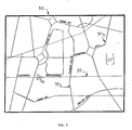
- Fig. 3 shows the map M of a given area (part of the map data base) or navigation neighborhood having a set of streets ⁇ St ⁇ over which the vehicle V may move.
- the street identified as "Lawrence Expressway” may correspond to a street St l
- the street identified as “Tasman Drive” may correspond to a street St 2
- the street identified as "Stanton Avenue” may correspond to a street St 3 .
- the vehicle symbol S which is displayed on the monitor 38.
- the vehicle V may move along Lawrence Expressway, then make a left turn onto Tasman Drive and then bear right onto Stanton Avenue, and this track will be seen by the vehicle operator via the relative movement of the symbol S v and map M.
- the map M is stored on the storage medium 14 as part of the map data base which is accessed by the computer 12.
- This map data base includes, as will be further described, data identifying (1) a set of line segments ⁇ S ⁇ defining the set of streets ⁇ St ⁇ , (2) street widths W, (3) vertical slopes of the line segments S, (4) magnetic variation of the geographical area identified by the map M, (5) map accuracy estimates, and (6) street names and street addresses.
- Fig. 4A is used to explain the data stored on medium 14 that identify a set of line segments ⁇ S ⁇ defining the set of streets ⁇ St ⁇ .
- Each such street St is stored on the medium 14 as an algebraic representation of the street St.
- each street St is stored as one or more arc segments, or, more particularly, as one or more straight line segments S.
- each line segment S has two end points EP 1 and EP 2 which are defined by coordinates X 1 Y 1 and X 2 Y 2 , respectively, and it is these XY coordinate data that are stored on the medium 14.
- the course (heading) of the segment S can be determined from the end points.
- the streets St of any given map M may be of different widths W, such as a six-lane street like Lawrence Expressway, a four-lane street like Stanton Avenue and a two-lane street like Tasman Drive, all illustrated in the map M of Fig. 3.
- Data identifying the respective widths W of each street St are stored on the medium 14 as part of the map data base.
- the width W of the street St is used as part of an update calculation described more fully below.
- Fig. 4B is used to explain correction data relating to the vertical slope of a given street St and which are part of the map data base stored on medium 14.
- Fig. 4B-1 shows a profile of the actual height of a street St which extends over a hill. The height profile of the actual street St is divided into line parts P 1 -P 5 for ease of explanation, with each part P 1 -P 5 having a true length 1 1 -1 5 .
- Fig. 4B-2 shows the same parts P 1 -P S as they are depicted on a flat map M as line segments S 1 -S 5 . Parts P 1 , P 3 and P 5 shown in Fig.
- the map data base can store vertical slope correction data for these segments S 2 and S 4 to compensate for the foreshortening errors.
- the correction data may be stored in the form of a code defining several levels of slope. For example, in some places these slope data may be coded at each segment S. In other areas these slope data are not encoded in the segment S but may be coded to reflect overall map accuracy, as described below.
- Fig. 4B-3 is a plot of the heading H measured by the means 26 for each segment S 1 -S 5 as the vehicle V traverses the street St having the height profile shown in Fig. 4B-1.
- the map data base contains correction data for segment S vertical slope the compass heading errors also may be corrected.
- foreshortening coefficients C F are calculated from foreshortening and other data coded for the selected segment S, as is the corrected heading H'.
- the map data base may contain correction data to relate magnetic north to true north and magnetic dip angles to determine heading errors due to the vertical slope of streets St, thereby accounting for the actual magnetic variation of a given geographic area. Because these are continuous and slowly varying correction factors only a few factors need be stored for the entire map data base.
- the map M is subject to a variety of other errors including survey errors and photographic errors which may occur when surveying and photographing a given geographic area to make the map M, errors of outdated data such as a new street St that was paved subsequent to the making of the map M, and, as indicated above, a general class of errors encountered when describing a 3-dimensional earth surface as a 2-dimensional flat surface. Consequently, the map data base may contain data estimating the accuracy for the entire map M, for a subarea of the map M or for specific line segments S. The navigational algorithm described below may use these map accuracy data to set a minimum size of an estimate of the accuracy of the updated dead reckoned position DRP also as described more fully below.
- some streets St in the map M are known to be generalizations of the actual locations (e.g., some trailer park roads).
- the map accuracy data may be coded in such a way as to identify these streets St and disallow the navigational algorithm from updating to these generalized streets St.
- the present invention provides information on the current dead reckoned position DRP of the vehicle V by using certain sensor data about wheel sensors 18 and compass 28 and the computations of equations (1) and (2) or (1') and (2').
- sensor calibration information derived in the process of advancing and updating the dead reckoned positions DRP, as will be described below, is used to improve the accuracy of such sensor data and, hence, the dead reckoned position accuracy.
- the present invention provides and maintains or carries forward as the vehicle V moves, an estimate of the accuracy of any given dead reckoned position DRP. Every time the dead reckoned position DRP is changed, i.e., either advanced from the old dead reckoned position DRP to the current dead reckoned position DRP c or updated from the DRP c to the updated current dead reckoned position DRP , the estimate is changed to reflect the change in the accuracy of the DRP.
- the estimate embodies the concept that the actual location of the vehicle V is never precisely known, so that the estimate covers an area that the vehicle V is likely to be within.
- the estimate of the accuracy of a given dead reckoned position DRP can be implemented in a variety of forms and is used to determine the probability of potential update positions of a given DRP c to a DRP cu .
- Fig. 5A generally is a replot of Fig. 1B on an XYZ coordinate system, where the Z axis depicts graphically a probability density function PDF of the actual location of the vehicle V.
- Fig. 5A shows along the XY plane the street St, together with the locations Land L and the current dead reckoned position DRP previously described in connection with Fig. 1B.
- the peak P of the probability density function PDF is situated directly above the DRP .
- the probability density function PDF is shown as having a number of contours each generated by a horizontal or XY plane slicing through the PDF function at some level. These contours represent contours of equal probability CEP, with each enclosing a percentage of the probability density, such as 50% or 90%, as shown.
- Fig. 5B is a projection of the contours CEP of Fig. 5A onto the XY coordinates of the map M.
- a given contour CEP encloses an area A having a certain probability of including the actual location of the vehicle V.
- the 90% contour CEP encloses an area A which has a 0.9 probability of including the actual location of the vehicle V.
- the area A of the CEP will become proportionately larger to reflect the accumulation of the error E and the resulting reduction in the accuracy of the DRP ; however, when the DRP is updated to the DRP , as was described in connection with Fig. 1C, then the area A of the CEP will be proportionately reduced to reflect the resulting increase in the accuracy of the DRP .
- the CEP still represents a constant probability of including the actual location of the vehicle V. As will be described, the CEP has a rate of growth or expansion which will change, accordingly, as certain measurements and other estimates change.
- Fig. 5C is similar to Fig. 5B, except that it shows one example of a specific implementation of the CEP that is used in accordance with the present invention, as will be further described.
- a contour CEP is approximated by a rectangle having corners RSTU.
- the CEP is stored and processed by the computer 12 as XY coordinate data defining the corners RSTU, respectively.
- the CEP whether stored and used in an elliptical, rectangular or other such shape, may be considered to constitute a plurality of points, each identified by XY coordinate data, defining a shape enclosing an area A having a probability of including the actual location of the vehicle V.
- Fig. 5C-1 shows graphically the expansion or enlargement of the CEP as the vehicle V moves over a street St and as an old dead reckoned position DRP o is advanced to a current dead reckoned position DRP.
- a given DRP is shown as not necessarily coinciding with an actual location L of the vehicle V, i.e., there is an accumulation error E.
- the CEP Surrounding the DRP o is the CEP having an area A that is shown as containing the actual location L o of the vehicle V.
- the CEP Upon the advancement of the DRP to the DRP , when the vehicle V has moved to the location L c , the CEP will have been expanded from the area A defined by corners RSTU to the area A' defined by corners R'S'T'U'. More specifically, as the vehicle V moves from the location L to the location L c , the computer 12 processes certain data so that the CEP may grow from area A to area A' at a varying rate, as will be described below. Also, the manner in which the XY coordinate data of the corners RSTU are changed to define corners R'S'T'U' will be described below.
- Fig. 5C-2 shows graphically the reduction in size of the CEP.
- Fig. 5C-2 indicates that at the time the vehicle V is at the location L , the vehicle navigational algorithm of the present invention has determined that a more probable current position than the DRP exists, so that the latter has been updated to the DRP , as explained in Fig. 1C. Consequently, the expanded CEP having corners R'S'T'U' is also updated to a CEP having an area A" with corners R"S"T"U" to reflect the increased certainty in the accuracy of the DRP cu . Again, the CEP having the area A" surrounds the DRP cu with a probability of including the actual location of the vehicle V. The detailed manner in which the CEP is updated to the CEP by the computer 12 will be described more fully below.
- the estimate of the accuracy of a given dead reckoned position DRP which has a probability of containing the actual location of the vehicle V, may be implemented in embodiments other than the CEP.
- the estimate may be a set of mathematical equations defining the PDF. Equation A is an example of a PDF of a DRP advancement assuming independent zero mean normal distributions of errors in heading and distance, and to first order approximation, independence of errors in the orthogonal directions parallel and perpendicular to the true heading direction.
- Equation B is an example of a similar PDF of the accumulated error. Its axes, ⁇ and ⁇ , have an arbitrary relation to D and P depending upon the vehicle's past track.
- the vehicle position probability density function PDF after an advance can be calculated by two dimension convolution of the old PDF (equation B) and the current PDF (equation A) and their respective headings.
- a new PDF of the form of equation B could then be approximated with, in general, a rotation of axis ⁇ to some new axis ⁇ ' and ⁇ to ⁇ ' and an adjustment of ⁇ ⁇ and ⁇ ⁇ .
- the computer 12 can then calculate the probability of potential update positions in accordance with these mathematical PDF equations thus providing information similar to that of the CEP as the vehicle V moves.
- the computer 12 can store in memory a table of values defining in two dimensions the probability distribution.
- the table can be processed to find similar information to that contained in the CEP, as described more fully below.
- the rate of growth of the CEP can be embodied in different ways. Besides the method described below, the rate of growth could be embodied by a variety of linear filtering techniques including Kalman filtering.
- Computer 12 will derive and evaluate from the above-described information one or more parameters that may be used to determine if a more probable position than the current dead reckoned position DRP exists.
- These "multi-parameters”, any one or more of which may be used in the determination, include (1) the calculated heading H of the vehicle V in comparison to the headings of the line segments S, (2) the closeness of the current dead reckoned position DRP to the line segments S in dependence on the estimate of the accuracy of the DRP , such as the CEP in the specific example described above, (3) the connectivity of the line segments S to the line segment S corresponding to a preceding DRP , (4) the closeness of the line segments S to one another (also discussed below as "ambiguity") , and (5) the correlation of the characteristics of a given street St, particularly the headings or path of the line segments S of the given street St, with the calculated headings H which represent the path of the vehicle V.
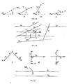
- Figs. 6A-6D show graphically and are used to explain the parameters (1)-(4) derived by
- Fig. 6A shows in illustration I the measured heading H of the vehicle V.
- Fig. 6A also shows in respective illustrations II-IV a plurality of line segments S, for example line segments S 1 -S 3 , stored in the map data base. These segments S 1 -S 3 may have, as shown, different headings h 1 -h 3 , as may be calculated from the XY coordinate data of their respective end points EP.
- the heading H of the vehicle V is compared to the respective headings h of each segment S in the map data base corresponding to the navigation neighborhood currently used by the navigation algorithm, such as segments S 1 -S 3 .
- computer 12 determines if one or more of these segments S qualifies as a "line-of-position" or L-O-P in determining if a more probable current dead reckoned position DRP exists. Such segments S qualifying as L-O-Ps are candidates for further consideration to determine if a DRP c is to be updated to DRP cu .
- Fig. 6B is used to explain one example of the closeness parameter with respect to the estimate of the accuracy of the DRP.
- one criterion that is considered is whether a given line segment S intersects or is within the CEP. Segments S intersecting the CEP are more likely to correspond to the actual location of the vehicle V than segments S not intersecting the CEP.
- a given line segment S doesn't intersect the CEP if, for example, all four corners RSTU (or R'S'T'U') are on one side of the CEP. As shown in Fig.
- FIG. 6B which illustrates eight representative line segments S 1 -S 8 , segments S 2 -S 4 and S 6 -S 7 (S 6 and S 7 correspond to one given street St) do not intersect the CEP and, therefore, are not considered further. Segments S 1 , S 5 and S 8 do intersect the CEP and, therefore, qualify as L-O-Ps or candidates for further consideration in determining if a more probable current dead reckoned position DRP exists, as will be described below.
- Fig. 6B happens to show that the actual location of the vehicle V at this time is on a street St corresponding to segment S 8 .
- the embodiment of the estimate being used is the table of entries of values of the probability density function PDF described above.
- the computer 12 may determine the distance and heading between a given line segment S and the DRP . From this and the table of PDF's the computer 12 can determine the most probable position along the segment S and the probability associated with that position. Any probability less than a threshold will result in the given line segment S not being close enough to the current dead reckoned position DRP to be a likely street St on which the vehicle V may be moving, whereas any probability greater than the threshold may constitute such a likely street St.
- these probability values can be used to rank the relative closeness of candidate segments S.
- a given line segment S corresponds to a street St on which the vehicle V is moving if it is connected to a line segment S previously determined to contain the updated current dead reckoned position DRP cu .
- Fig. 6C graphically illustrates several possible ways in which two line segments S 1 and S 2 are deemed connected. As shown in Example I of Fig. 6C, any two line segments S 1 and S 2 are connected if an intersection i of these two segments S 1 and S 2 is within a threshold distance of the end points EP of the two segments S 1 , and S 2 , respectively. Alternatively, two line segments S 1 and S 2 are interconnected if the intersection i is inclusive of the end points EP, as shown by Example II and Example III in Fig. 6C.
- the line segment S 1 may be the segment S corresponding to the preceding updated current dead reckoned position DRP cu while line segment S 2 may be a segment S being presently evaluated in connection with updating the current dead reckoned position DRP.
- Computer 12 will compute from segment data contained in the navigation neighborhood of the map data base, the connectivity to determine if this segment S 2 qualifies under this connectivity test. That is, the present invention considers that the vehicle V more likely will move about interconnected streets St and line segments S of a given street St, rather than about unconnected streets St or unconnected line segments S of a given street St. Other segments S may or may not so qualify under this connectivity parameter. Since the present invention also allows for the vehicle V to move off and on the set of streets S of the map data base, this connectivity test is not absolute but is one of the parameters used in the updating process more fully described later.
- Fig. 6D shows two line segments S 1 and S 2 on opposite sides of the current dead reckoned position DRP c .
- the computer 12 ultimately may determine that these two line segments S 1 and S 2 are the only two remaining line segments S that may likely correspond to the actual street St on which the vehicle V is moving. However, if the computer 12 determines that these two segments S 1 and S 2 are too close together, or that the distance between S 1 and DRP c is insignificantly different than the distance between S 2 and D RP , then one segment S 1 or S 2 may be as likely as the other segment S 1 or S 2 to correspond to the street St on which the vehicle V is actually moving. In this ambiguous event, neither segment S 1 nor S 2 is selected as a more probable segment and the current dead reckoned position DRP is not updated at this time.
- the correlation parameter generally describes the closeness of fit of a recent portion of the path taken by the vehicle V to the path defined by segments S in the navigation neighborhood.
- the correlation parameter is computed differently depending upon whether the vehicle V is turning or not. If the vehicle V is not turning a simple path matching is calculated, as described below in section 5(b). If the vehicle V is turning a correlation function is calculated, as described below in section 5(c).
- path matching is used when the vehicle V has been determined not to be turning.
- the solid lines having the current dead reckoned position DRP show a recent dead reckoned path used for matching and the dashed lines show an older dead reckoned path not used for matching.
- the other solid lines of examples I and II show respective sequences of connected line segments S.
- Example I of Fig. 6E shows paths that do match, whereby segment S 2 would be used for updating the current dead reckoned position DRP to the DRP .
- Example II shows paths that do not match, so that segment S 2 would not be used for updating the current dead reckoned position DRP .
- a correlation function is used when it has been determined that the vehicle V has been turning.
- the correlation function is derived to determine if the segment S is sufficiently correlated to warrant updating the current dead reckoned position DRP.
- the computer 12 does this by calculating the best point BP of the correlation function and testing its value as well as certain shape factors. If it passes these tests, this best point BP is stored for later use in updating the DRP to DRP cu .
- Section IV the parameters of Section IV. discussed above are used as logical tests in conjunction with other processing and logical tests to determine if a point along a selected segment S, i.e., the most probable segment, is a more probable position of the vehicle V than the current dead reckoned position DRP. If such a most probable segment S is selected, then an update of the DRP to that point (the DRP ) will be made as outlined in Section VI. below and detailed more fully in Section IX.
- the parameters are generally used to sequentially test and eliminate the set of segments S in the navigation neighborhood from further consideration as candidate segments S for the most probable segment S.
- the navigation algorithm uses these parameters and other processing and logic to eliminate all but one or two segments S as candidate segments.
- the algorithm then makes a final determination if one segment S fully qualifies as having the highest probability of representing the street St where the vehicle V is moving and that the probability is sufficiently high to qualify for updating the current dead reckoned position DRP to the DRP cu as the above-mentioned point on such one segment S.
- these parameters for determining if and how to update the current dead reckoned position DRP can take other embodiments.
- they may be used in a weighted score algorithm.
- the parameters described in Section IV. above may be numerically computed for each segment S in the navigation neighborhood.
- Each parameter could be weighted by numerical values representing the average error bounds estimated for that parameter and representing the significance assigned to that parameter. In this way a weighted sum of scores could be computed for each segment S and the segment S with the best weighted sum determined. If that sum was sufficiently good the decision would be made to update.
- the computer 12 processes the segment, parameter and DRP data to determine the most probable DRP , the updated CEP and, if appropriate, updated distance and heading sensor calibration coefficients.
- the method of calculating DRP cu depends on whether the computer 12 determines that the vehicle V has been turning or has been moving in a straight line.
- DRP cu is computed directly using the selected segment S, the DRP , the angle and distance between them and the CEP. If the vehicle V is turning, the DRP cu is determined by calculating a correlation function obtained by comparing the sequence of recent vehicle headings to the segment S (and if necessary connected segments S). The best point BP of the correlation computation becomes the selected DRP cu if it passes certain quality tests.
- the CEP is updated to CEP differently in accordance with the two methods of updating the DRP . Also, when the update is judged to provide added information about the calibration of the sensors 18 and 28, the calibration coefficients are updated.
- the method of updating DRP c to DRP cu can take other embodiments.
- the past DRP positions, the most probable position along the selected segment S, the score of the segment S if a score was computed, as well as other parameter information could be input into a linear filter (not shown) for computing an optimum or least mean square position based on some assignment of values of the different inputs.
- the optimum or most probable position may or may not fall on a segment S.
- This information includes, for example, the distance and heading data inputted to the computer 12, the map data base stored on medium 14 and the estimate of the accuracy of the dead reckoned positions DRP.
- the computer 12 may use this information to derive one or more parameters, each of which and all of which, are useful for determining if a most probable segment S exists and if such segment S contains a more probable current dead reckoned position DRP than the current DRP .
- the computer 12 computes a more probable position and then updates the DRP to a DRP , the estimate c cu of the accuracy of the DRP and the calibration coefficients.
- the computer 12 may selectively process the information described and other information to be described, and derive the parameters, and perform the updates in accordance with a vehicle navigational algorithm of the present invention, one embodiment of which will now be described.
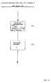
- Figs. 7A-7C show three block diagrams which, together, constitute an overall computer program structure that is utilized by the system 10.
- Fig. 7A references a main program, with Figs. 7B-7C referencing interrupt programs.
- the interrupt program of Fig. 7B is used to refresh the monitor 38 and to provide an operator interface via the console means 46.
- the interrupt program of Fig. 7C is the program performing the vehicle navigational algorithm of the present invention.
- the main program computes and formats data necessary to select and display the selected map M and the vehicle symbol S shown on the monitor 38 and provide the segments S in the navigation neighborhood for the vehicle navigational algorithm.
- the execution of this main program can be interrupted by the two additional programs of Fig. 7B and Fig. 7C.
- the refresh display program of Fig. 7B resets the commands necessary to maintain the visual images shown on the monitor 38 and reads in any operator command data via the console means 44 needed for the main program to select and format the display presentation.
- the interrupt program of Fig. 7B can interrupt either the main program of Fig. 7A or the navigational program of Fig. 7C. The latter can only interrupt the main program and does so approximately every 1 second, as will be further described.
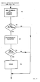
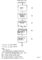
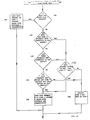
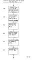
- Fig. 8 is a flow chart illustrating an embodiment of the overall vehicle navigational algorithm of the present invention performed by the computer 12.
- the computer 12 advances an old dead reckoned position DRP to a current dead reckoned position DRP by dead reckoning (see also Fig. 1B) and expands an estimate of the accuracy of the DRP (see also Fig. 5C-1) and (block 8A), as described further below in relation to Fig. 9.
- a decision is made if it is time to test for an update of the DRP , the estimate and other information (block 8B), as described below in relation to Fig. 12. If not, the remaining program is bypassed and control is returned to the main program.
- a multi-parameter evaluation is performed by computer 12 to determine if a segment S in the navigation neighborhood contains a point which is more likely than the current dead reckoned position DRP (block 8C), as will be described in relation to Fig. 13. If the multi-parameter evaluation does not result in the determination of such a segment S (block 8D), then the remaining program is bypassed and control is passed to the main program. If the multi-parameter evaluation indicates that such a more likely segment S does exist, then a position along this segment S is determined and an update is performed (block 8E), as will be described in connection with Fig. 28, and thereafter control is returned to the main program.
- This update not only includes an update of the current dead reckoned position DRP c to the DRP cu (see Fig. 1C), and an update of the estimate (see Fig. 5C-2), but also, if appropriate, an update of calibration data relating to the distance sensor means 16 and the heading sensor means 26 (see Fig. 2).
- Fig. 9 shows a flow chart of the subroutine for advancing the DRP o to DRP c and expanding the estimate of the accuracy of the DRP c (see block 8A).
- the DRP is advanced by dead reckoning to the DRP c (block 9A), as will be described in relation to Fig. 10.
- the estimate of the accuracy of the DRP c is enlarged or expanded (block 9B), as will be described in connection with Fig. 11.
- Fig. 10 illustrates the flow chart of the subroutine for advancing a given DRP o to the DRP (see block 9A).
- the heading H of the vehicle V is measured by computer 12 (block 10A), which receives the heading data from the sensor means 26.
- the measured heading H is then corrected for certain errors (block 10B). That is, and as will be described in relation to Fig. 35-1, the computer 12 maintains a sensor deviation table by storing heading sensor deviation vs. sensor reading, which heading deviation is added to the output of the heading sensor means 26 to arrive at a more precise magnetic bearing.
- the local magnetic variation from the map data base is added to the output of the heading sensor means 26 to arrive at a more accurate heading H of the vehicle V.
- a distance ⁇ d traveled since the calculation of the DRP o is measured by the computer 12 using the distance data from sensor means 18 (block 10C).
- the computer 12 calculates the distance ⁇ D (see Fig. 1B) (block 10D), in which the calibration coefficient C D is described more fully in relation to Fig. 35-2.
- the DRP is calculated using equations 1' and 2' (block 10E), and this subroutine is then completed.
- Fig. 11 discloses a flow chart of the subroutine for expanding the contour CEP (see block 9B). Reference also will be made to Fig. 11A which is a simplification of Fig. 5C-1 and which shows the enlarged CEP having area A' after the vehicle V has traveled from one location to another and the distance ⁇ D has been calculated.
- the X and Y distance components of the calculated ⁇ D are determined by the computer 12, as follows (block 11A):
- the computer 12 calculates certain variable heading and distance errors F H and E D , respectively, to be described in detail below.
- these errors E H and E D relate to sensor accuracies and overall system performance.
- E H and F D are variables, as are ⁇ D x and ⁇ D y since these data depend on the distance traveled by vehicle v from one location to the other when it is time to advance the DRP o and expand the CEP. Consequently, the rate at which the CEP expands will vary. For example, the higher the values for F H or F D , the faster the CEP will grow, reflecting the decreased accuracy of the DRP c and certainty of knowing the actual location of the vehicle V.
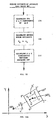
- Fig. 12 illustrates the flow chart of the subroutine for determining if it is time to test for an update (see block 8B) .
- the computer 12 determines if 2 seconds have elapsed since a previous update was considered (not necessarily made) (block 12A). If not, it is not time for testing for an update (block 12P) and the remaining program is bypassed with control being returned to the main program.
- computer 12 determines if the vehicle V has traveled a threshold distance since the previous update was considered (block 12C) . If not, it is not time for testing for an update (block 12B). If yes, then it is time to determine if an update should be made (block 12D).
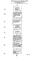
- Fig. 13 is a flow chart of the subroutine for performing the multi-parameter evaluation by the computer 12 (see blocks 8C and 8D).
- the computer 12 determines a most probable line segment S, if any, based on the parameters (1)- (4) Jisted above (block 13A), as will be further described in relation to Fig. 14. If a most probable line segment S has been found (block 13B), then a determination is made (block 13C) as to whether this most probable segment S passes the correlation tests of the correlation parameter, as will be described in relation to Fig. 23. If not, a flag is set to bypass the update subroutine (block 13D). If yes, a flag is set (block 13E), so that control proceeds to the update subroutines.
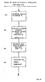
- Fig. 14 shows the flow chart of the subroutine for determining the most probable line segment S and if this line segment S is sufficiently probable to proceed with the update subroutines (see block 13A).
- the XY coordinate data of a line segment S are fetched by computer 12 from the navigation neighborhood of the map data base stored on medium 14 (block 14A).
- the computer 12 determines if this line segment S is parallel to the heading H of the vehicle within a threshold (see the heading parameter, Section IV Bl.) (block 14B), as will be described in relation to Fig. 15. If not, then the computer 12 determines if this line segment S is the last segment S in the navigation neighborhood to fetch (block 14C). If not, then the subroutine returns to block 14A, whereby the computer 12 fetches another segment S.
- the computer 12 determines if this line segment S intersects the CEP (block 14D) (see the closeness parameter relative to the estimate of the accuracy of the DRP ; Section IV B2).
- An example of a procedure for determining whether a line segment S intersects the CEP is disclosed in a book entitled, "Al.gorithms for Graphics and Image Processing," by Theodosios Pavlidis, Computer Science Press, Inc., 1982 at ⁇ 15.2 entitled, "Clipping a Line Segment by a Convex Polygon", and ⁇ 15.3 entitled, "Clipping a Line Segment by a Regular Rectangle".
- this line segment S does not intersect the CEP (block 14D) , and if this line segment S is not the last segment S in the navigation neighborhood that is fetched (block 14C), then the subroutine returns to block 14A, whereby the computer 12 fetches another line segment S. If this line segment S does intersect the CEP (block 14D), then this line segment S is added by the computer 12 to a list stored in memory of lines-of-position I-O-P (block 14E) which quality as probable segments S for further consideration.
- the computer 12 tests this line segment S which was added to the list for the parameters of cennectivity (see Section IV B3) and the closeness of twc line segments S (see Section IV B4) (block 14F) , as will be further described in relation to Fig. 16. If this line segment S fails a particular combination of these two tests, it is removed from the L-O-P list. The subroutine then continues to block 14C.
- chen a most probable line segment S is selected by the computer 12 from the remaining entries in the I.-O-P list (block 14G) , as will be further described in relation to Fig. 20. It is this selected most probable line segment S which is the segment to which the DRP is updated to the DRP cu if it passes the tests of the correlation parameter.
- Fig. 15 shows the flow chart of the subroutine for determining if a segment S is parallel to the headinq H of the vehicle V, i.e., the heading parameter (see block 14B).
- an angle ⁇ of the line segment S is calculated (block 15A) in accordance with the following equation: where X 1 , X 2 , Y 1 , Y 2 are the XY coordinate data of the end points EP of the line segment S currently being processed by the computer 12.
- the current heading H of the vehicle V is determined, i.e., the angle a (block 15B) from the heading data received from the sensor means 26.
- the computer 12 determines if
- Fig. 16 shows the flow chart of the subroutine for testing for the parameters of connectivity and closeness of two line segments S (see block 14F).
- the computer 12 calculates the distance from the current dead reckoned position DRP c to the line segment S (now a line-of-position L-O-P via block 14E) being processed (block 16A), as will be described further in relation to Fig. 17.
- the computer 12 accesses the navigation neighborhood of the map data base to compute if this line segment S is connected to the "old street", which, as previously mentioned, corresponds to the line segment S to which the next preceding DRP cu was calculated to be on (block 16B).
- This line segment S and the old street segment S are or are not connected, as was described previously in relation to Fig. 6C.
- this line segment S currently being processed is not the first segment S (block 16C)
- the computer 12 determines if this segment S is on the same side of the DRP as the side 1 segment S (block 16G). If it is on the same side as the side 1 segment S, then the computer 12 selects the most probable segment S on side 1 (block 16H), as will be described in relation to the subroutine of Fig. 18.
- this line segment S is not on side 1 (block 16G), then it is on "side 2", i.e., the other side of the DRP. Accordingly, the most probable segment S on side 2 is selected (block 16I), as will be described for the subroutine of Fig. 19.
- a most probable line segment S if any on side 1 and a most probable line segment S if any on side 2 of the DRP have been selected, and these will be further tested for closeness or ambiguity, as will be described in relation to Fig. 20. All other L-O-P's on the list (see block 14E) have been eliminated from further consideration.
- Fig. 17 is a flow chart showing the subroutine for calculating a distance d from the DRP c to a line segment S (see block 16A).
- the intersection I of a line 1 perpendicular to the segment S, and the segment S is calculated by the computer 12 (block 17A).
- the reason for the perpendicularity of the line 1 is that this will provide the closest intersection I to the DRP.
- This intersection I is identified by coordinate data X 3 Y 3 .
- the distance d between the DRP and the intersection I is calculated using the XY coordinate data of the DRP c and X 3 Y 3 (block 17B).
- Fig. 18 illustrates the flow chart of the subroutine for selecting the most probable line segment S on side 1 of the current dead reckoned position DRP c (see block 16H).
- the computer 12 determines if this line segment S being processed and the side 1 line segment S are both connected to the old street segment S (block 18A). If so connected, then the computer 12, having saved the result of the distance calculation (block 16E), determines if this line segment S is closer to the current dead reckoned position DRP c than the side 1 line segment S (block 18B). If not, the side 1 segment S is retained as the side 1 segment S (block 18C). If closer, then this line segment S is saved as the new side 1 segment S along with its distance and connectivity data (block 18D).
- the computer 12 determines if this line segment S and the side 1 segment S are not both connected to the old street segment S (block 18E). If the answer is y es, then the subroutine proceeds via block 18B as above. If the answer is no, then the computer 12 determines if this line segment S is connected to the old street segment S and if the side 1 segment S is not so connected (block 18F). If the answer is no, then the side 1 segment S is retained as the side 1 segment S (block 18C). Otherwise, this line segment S becomes the side 1 segment S (block 18D). Thus, at the end of this subroutine, only one line segment S on one side of the current dead reckoned position DRP is saved as the side 1 segment S.
- Fig. 19 shows the flow chart of the subroutine for selecting the most probable line segment S on side 2, i.e., the other side from side 1 of the current dead reckoned position DRP c (see block 16I). If this is the first line segment S on side 2 being considered by the computer 12 (block 19A), then this line segment S is saved as the "side 2" segment S along with its distance and connectivity data (block 19B). If not, then the computer 12, having saved the results of the street connection tests (block 16F), decides if this line segment S and the side 2 segment S are both connected to the old street segment S (block 19C).
- the computer 12 having saved the results of the distance calculation (block 16E), decides if this line segment S is closer to the current dead reckoned position DRP than the side 2 segment S (block 19D). If not, the side 2 segment S is retained as the side 2 segment S (block 19E). If it is closer, then this line segment S is now saved as the side 2 segment S along with its distance and connectivity data (block 19F).
- the computer 12 determines if this line segment S and the side 2 segment S are both not connected to the old street segment S (block 19G). If the answer is yes, then the subroutine proceeds through block 19D. If not, then a decision is made by the computer 12 if this line segment S is connected to the old street segment S and the side 2 segment S is not connected to the old street segment S (block 19H). If not, then the side 2 segment S is retained as the side 2 segment S (block 19E). If yes, then this line segment S is retained as the new side 2 segment S along with its distance and connectivity data (block 19F).
- Fig. 20 shows the flow chart of the subroutine for selecting the most probable segment S of the remaining segments S (see block 14G).
- the computer 12 having made a list of segments S qualifying as a line-of-position L-O-P (block 14E) and eliminating all but no more than two, determines if only one segment S has qualified as such a line-of-position L-O-P (block 20A). If there is only one, then this line segment S is selected as the most probable segment S in the navigation neighborhood at this time (block 20B). The computer 12 then determines if this most probable segment S passes the tests of the correlation parameter (block 20C), as will be described in connection with the subroutine of Fig. 23. If this segment S does not pass these tests, no update will occur. If this segment S passes the correlation tests, then the subroutine continues accordingly towards determining the point on this line segment S to which the DRP cu should be positioned, i.e., towards an update of DRP to DRP . c cu
- the computer 12 determines if the side 2 segment S is connected to the old street segment S and the side 1 segment S is not connected to the old street segment S (block 20F). If the answer is yes, then the side 2 segment S is selected as the most probable segment S in the navigation neighborhood (block 20G), and the subroutine continues directly to block 20C. If the answer is no, then the computer 12 determines if the side 1 segment S and the side 2 segment S are too close together (block 20H) (see the ambiguity parameter; Section IV B4), as will be described more fully in relation to the flow chart of Fig. 21. If the side 1 segment S and the side 2 segment S are too close together, then the computer 12 determines that no most probable segment S exists at this time (block 201) and no update will be made at this time.
- the computer 12 determines if one segment S is closer to the DRP than the other segment S within a threshold (block 20J), as will be further described in connection with the subroutine of Fig. 22. If not, then the computer 12 determines that no most probable segment S occurs at this time (block 201); consequently, no update will be made at this time. If yes, then the one segment S is selected as the most probable segment S (block 20K) and the subroutine continues to block 20C. Thus, at the completion of this subroutine, either no most probable segment S exists at this time or a most probable segment S exists if it passes the test of the correlation parameter (see Section IV.B.5 above).
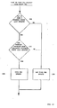
- Fig. 21 shows the flow chart of the subroutine for determining if the side 1 and side 2 segments S are too close together (see block 20H).
- the distance between the two segments S is calculated by the computer 12 (block 21A).
- the computer 12 determines if this distance is below a threshold distance (block 21B). If yes, then the two segments S are too close together, representing an ambiguous condition (block 21C), thereby resulting in no updating at this time. If not, the segments S are determined to be not too close together (block 21D) and an update possibly may occur.
- Fig. 22 illustrates the flow chart of the subroutine for determining if the side 1 segment S or the side 2 segment S is significantly closer to the DRP than the other (see block 20J).
- the computer 12 calculates the ratio of the distance from the DRP c to the side 1 segment S to the distance from the DRP to the side 2 segment S (block 22A). Then, the computer 12 determines if this ratio is greater than a threshold or less than 1/threshold, (block 22B). If not, then the DRP is determined to be not closer to one segment S than the other segment S (block 22C), thereby resulting in no updating at this time. If yes, then the DRP is determined to be closer to the one segment S than the other (block 22D) and an update possibly may occur.
- Fig. 23 shows the subroutine for performing the correlation tests with respect to the most probable segment S (see block 20C).
- a determination is made by the computer 12 as to whether or not the vehicle has been turning, as will be described further in relation to Fig. 25. If the computer 12 determines that the vehicle V has not been turning (block 23A), it performs the correlation test by a simple path matching computation (blocks 23B-23F), as will be described in conjunction with Figs. 24A-24D (see also Section IV.B.5b above). Otherwise, it performs the correlation test by calculating and testing a correlation function (blocks 23G-23J) (see also Section IV.B.5c above).
- Fig. 24A to Fig. 24D are illustrations of plots of various data used by the computer 12 in determining if the simple path match exists.
- Fig. 24A is a plot of XY positions of a plurality of segments S of the street St on which the vehicle V may be actually moving, in which this street St has six line segments S 1 -S 6 defined by end points a-g, as shown, and one of which corresponds to the most probable segment S.
- Fig. 24B is a plot of the XY positions of a plurality of dead reckoned positions DRP previously calculated in accordance with the present invention and equations (1) or (1') and (2) or (2'), as shown at points A-K, including the current dead reckoned position DRP at point K.
- Fig. 24A is a plot of XY positions of a plurality of segments S of the street St on which the vehicle V may be actually moving, in which this street St has six line segments S 1 -S 6 defined by end points a-g, as shown, and
- Fig. 24B shows these dead reckoned positions DRP over a total calculated distance D traveled by the vehicle V, which is the sum of ⁇ D 1 - ⁇ D 10 .
- Fig. 24C shows the headings h l -h 6 corresponding to the line segments S 1 -S 6 , respectively, as a function of distance along the street St of Fig. 24A (as distinct from the X position).
- the map data base has end point data identifying the line segments S 1 -S 6 of a given street St shown in Fig. 24A, but the heading data of Fig. 24C are calculated by the computer 12, as needed in accordance with the discussion below.
- Fig. 24D shows the corresponding measured headings H 1 -H 10 of the vehicle V for ⁇ D 1 - ⁇ D 10 , respectively, of Fig. 24B.
- the AD distance data and the heading data H 1 -H 10 shown in Fig. 24B and Fig. 24D are calculated by and temporarily stored in the computer 12 as a heading table of entries.
- Fig. 24D is a plot of this table. Specifically, as the vehicle V travels, every second the distance traveled and heading of the vehicle V are measured. An entry is made into the heading table if the vehicle V has traveled more than a threshold distance since the preceding entry of the table was made.
- the computer 12 calculates the heading h of the street St for each entry in the heading table for a past threshold distance traveled by the vehicle V (block 23B). That is, this heading h of the street St is calculated for a threshold distance traveled by the vehicle V preceding the current dead reckoned position DRP indicated in Fig. 24B. For example, this threshold distance may be approximately 300 ft.
- the computer 12 calculates the RMS (root mean square) heading error over this threshold distance (block 23C).
- the computer 12 determines if this RMS heading error (calculated for one position p - the DRP ) is less than a threshold (block 23D). If it is, then the computer 12 determines that the measured dead reckoning path of the vehicle V does match this most probable segment S and the latter is saved (block 23E). If not, then the computer 12 determines that the measured dead reckoning path of the vehicle V does not match this most probable segment, so that there is no most probable segment S (block 23F). Thus, if the match exists, there is a most probable segment S to which the current dead reckoned position DRP can be updated; otherwise, no update is performed at this time.
- the computer 12 determines that the vehicle V has been turning (block 23A), then it performs the correlation test by computation of a correlation function (blocks 23G-23J).
- the computer 12 calculates a correlation function between the measured path of the vehicle V and the headings of certain line segments S including the most probable segment S and line segments S connected to it (block 23G), as will be described further in relation to Fig. 26.
- the computer 12 determines if the results from this correlation function passes certain threshold tests (block 23H), as will be described in relation to Fig. 27. If not, then no most probable segment is found (block 23F).
- Fig. 25 shows the subroutine for determining if the vehicle V is turning (see block 23A).
- the computer 12 begins by comparing the data identifying the heading H associated with the current dead reckoned position DRP and the data identifying the preceding heading H associated with the old dead reckoned position DRP (block 25A). If the current heading data indicate that the current heading H has changed more than a threshold number of degrees (block 25B), then the computer 12 decides that the vehicle V has been turning (block 25C).
- the computer 12 determines if the vehicle V has been on the current heading H for a threshold distance (block 25D). If not, the vehicle V is determined to be turning (block 25C); however, if the vehicle V has been on the current heading H for a threshold distance (block 25D), then a decision is made by the computer 12 that the vehicle V is not turning (block 25E).
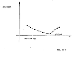
- Fig. 26 illustrates the flow chart of the subroutine for calculating the correlation function between the path of the vehicle V and the selected line segments S mentioned above (see block 23G), while Fig. 26-1 illustrates the calculated correlation function.
- the correlation function is calculated by first calculating a maximum dimension L of the CEP associated with the DRP (block 26A). c Then, with reference again to Fig. 24A and Fig. 24C, which are also used to explain this correlation test, the two end points EP 1 , EP 2 of the interval L which are plus or minus L/2 respectively from a best guess (BG) position for the DRP cu are calculated by the computer 12 (block 26B). Next, the computer 12 divides this interval L into a plurality of positions which are, for example, 40 feet apart (block 26C).
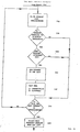
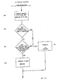
- Fig. 27 illustrates the flow chart of the subroutine for determining if the correlation function passes certain thresholds (see block 23H).
- the computer 12 finds the position of minimum RMS error (block 27A), which is shown in Fig. 26-1. Then, the computer 12 determines if this RMS error is below a threshold (block 27B). If not, the remaining subroutine is bypassed and no most probable segment S is found (returning to block 23F). If the RMS error is below a threshold, then the curvature of the correlation function at the minimum position is calculated by taking a second order difference of the RMS error vs. position (block 27C).
- this curvature is not above a threshold (block 27D), then the correlation test fails and the remaining subroutine is bypassed (block 27F). If this curvature is above the threshold (block 27D), then the computer 12 determines that the correlation calculation passes the test of all thresholds (block 27E), whereby the position of the RMS minimum error is the best point BP (see block 231) that becomes DRP . If the curvature is above the threshold, then this assures that the correlation parameter has peaked enough. For example, if the line segments S for the distances covered by the heading table are straight, then the second order difference would be zero and the correlation parameter would not contain any position information for the DRP cu
- Fig. 28 is a flow chart showing generally the subroutine for the update (see block 8E).
- the computer 12 updates the current dead reckoned position DRP to the current updated dead reckoned position DRP cu (block 28A), as will be further described in relation to Fig. 29.
- the computer 12 updates the estimate of the accuracy of the DRP c (block 28B), as will be described in relation to Fig. 32.
- the sensor means 16 and sensor means 26 are recalibrated (block 28C), as will be described in relation to Fig. 35.
- Fig. 29 illustrates the flow chart of the subroutine for updating the DRP to the DRP .
- the XY coordinate data of the DRP are set to the XY c coordinate data of the best correlation point BP previously calculated (see block 23I), thereby updating the DRP c to the DRP cu (block 29B).
- a dead reckoning performance ratio PR is calculated (block 29C), which, for example, is equal to the distance between the DRP c and the DRP cu divided by the calculated distance ⁇ D the vehicle V has traveled since the last update of a DRP to a DRP cu .
- This performance ratio PR is used to calculate a certain error in the system 10 that, as previously mentioned and as will be further described, is used for determining the varying rate or rate of growth of the CEP. If the vehicle V has not been turning (block 29A), then the DRP is set to the most probable constant course position (block 29D), as will be described in relation to Fig. 30, followed by the calculation of the dead reckoning performance ratio PR (block 29C).
- Fig. 30 illustrates the flow chart of the subroutine for updating a given DRP to a given DRP cu when the vehicle V is on a constant heading H (see block 29D).
- Fig. 30-1 also will be used to describe the updating of the DRP c to the DRP cu and shows the DRP , a given CEP associated with the DRP and the most probable line segment S.
- the computer 12 calculates the aspect ratio AR of the CEP, which equals
- the computer 12 calculates an angle a of the segment S shown in Fig. 30-1 (block 30D). Then, the computer 12 calculates an angle ⁇ of the major axis of the CEP, as shown in Fig. 30-1, (block 30E). Next, the computer 12 determines if the angle (a - ⁇ ) is less than a threshold (block 30F). If it is, then the subroutine proceeds to block 30C. If not, the DRP c is updated to a most probable point (approximately the most probable point) on the segment S (block 30G), as will now be described in relation to Fig. 31.
- Fig. 31 shows the flow chart of the subroutine for updating the DRP c to a most probable point on the most probable segment S (see block 30G).
- the computer 12 determines the sides which are parallel to the major axis of the CEP, i.e., sides S 1 and S 2 in the example shown in Fig. 30-1, (block 31A).
- the computer 12 calculates the points P 1 and P 2 where the sides S 1 and S 2 intersect the most probable segment S (block 31B).
- the computer 12 calculates the mid-point P 4 between point P 1 and P 2 (block 31C).
- the computer 12 calculates the closest point P 3 (block 31D) in the manner previously described.
- a distance d between point P3 and point P 4 is calculated by the computer 12 (block 31E).
- the computer 12 calculates the XY coordinate data of the DRP cu (block 31F) in accordance with the following equations:
- the computer 12 performs the subroutine shown in Fig. 32 for updating the CEP associated with the DRP c to an updated CEP u associated with the DRP cu (see block 28B). If the vehicle has not been turning (block 32A), then the CEP is updated based on the constant heading most probable position (block 32B), as will be described in Fig. 33. If the vehicle has been turning, the CEP will be updated based on the calculation of the correlation function (block 32C), as will be described in Fig. 34.
- Fig. 33 shows the flow chart of the subroutine for updating the CEP to the CEP u based on the constant heading most probable position (see block 32B). Also, reference will be made to Fig. 33-1 which is used to explain the flow chart of Fig. 33, in which Fig. 33-1 shows a given CEP, the associated DRP , the DRP and the resulting CEP .
- the computer 12 has calculated the DRP cu as described previously in relation to Fig. 30.
- an angle a of the most probable segment S is calculated (block 33A).
- the computer 12 calculates a line 1 1 which is parallel to the most probable segment S and passes through the DRP c (block 33B), i.e., line 1 1 also has the angle a.
- points P 1 and P 2 along the line 1 1 which intersect the CEP are calculated (block 33C).
- the computer 12 calculates the distance d 1 between the points P 1 and P 2 (block 33D).
- the computer 12 determines the half axis or distance d 3 for the CEP u perpendicular to the most probable segment S, in which d 3 is equal to the half-width of the width W of the street St that is fetched from the navigation neighborhood of the map data base (block 33F).
- the calculated distances, d 2 and d 3 are compared to threshold minimum distances according to the map accuracy data fetched from the map data base (block 33G) to set the minimum size of the CEP u (see Section III.A.2.f). Finally, the XY coordinate data of the corners R"S"T"U" of the CEP u are calculated as follows (block 33H):
- Fig. 34 shows the flow chart of the subroutine for updating the CEP to the CEP based on the outcome of correlation function (see block 32C).
- Fig. 34-1 which shows the most probable segment S, the DRP and the resulting CEP , will also be used to describe the flow chart of Fig. 34.
- the computer 12 calculates an angle a (block 34A).
- an estimated uncertainty of the position of the DRP based on the curvature of the correlation function is calculated, i.e., the distance d 2 (block 34B).
- the computer 12 determines the half-width, d 1 , of the street St based on its width W which is fetched from the navigation neighborhood of the map data base (block 34C).
- the calculated distances, d 1 and d 2 are compared to threshold minimum distances according to the map accuracy data fetched from the map data base to set the minimum size of the CEP u ; (see Section III.A.2f).
- the updated CEP u is calculated using similar equations as shown for R", as follows (block 34D):
- Fig. 35 now shows the flow chart of the subroutine for recalibrating the sensor means 16 and 26 (see block 28C). If the vehicle V is turning (block 35A), as may be determined in a manner previously described, then the remaining subroutine is bypassed and the sensor means 16 and 26 are not recalibrated at this time. If the vehicle V is not turning, then the heading sensor means 26 is recalibrated (block 35B), as will be described more fully below in relation to Fig. 35-1. Next, if the vehicle V did not just finish a turn, then the remaining subroutine is bypassed (block 35C). If the vehicle V did just finish a turn, then the distance sensor means 16 is recalibrated (block 35D), as will be described more fully below in relation to Fig. 35-2.
- Fig. 35-1 shows a plot of the deviation of the heading sensor means 26 as a function of the output of the heading sensor means 26.
- This plot is stored on medium 14 as a heading deviation table mentioned previously.
- the computer 12 can now make an appropriate correction in the heading deviation table corresponding to a particular output of the heading sensor means 26 to correct a corresponding calibration coefficient stored on medium 14 and, thereby, provide the more accurate advancement of a given DRP to a given DRP .
- Fig. 35-2 assume that the vehicle V is traveling on a street St 1 and makes a right turn onto the street St 2 . Assume also that after the turn onto the street St 2 , the calculation of the DRP places the vehicle V from position A to either position B, which is short of the street St 2 , or to position B' which is beyond the street St 2 . Also assume that as a result of the vehicle navigational algorithm, the DRP at position B or position B' is updated to position C which happens to coincide with the actual location of the vehicle V.
- the calibration of the distance sensor means 16 is checked after the vehicle V makes the turn onto the street St 2 .
- the calibration coefficient C D (see Fig. 10) of the distance sensor means 16 is increased or decreased, as follows. If the DRP c placed the position of the vehicle V short of the street St 2 within a threshold, as shown at point B, the calibration coefficient C D is too low and, therefore, increased. If, however, the DRP c placed the vehicle V beyond the street St 2 within a threshold, as shown at B', the calibration coefficient C D is too high and, therefore, is decreased. As with other calibration data, the distance calibration coefficient C D is stored on the medium 14 and processed by the computer 12 to provide a more accurate DRP.
- Fig. 36 is a flow chart of a subroutine for determining E H and E D .
- the computer 12 calculates a change in heading from information received from the flux gate compass 28 shown in Fig. 2 (block 36A), as a DRP is advanced to a DRP.
- the computer 12 calculates the change in heading from information received from the differential wheel sensors 18 of Fig. 2 (block 36B) as the DRP is advanced to the DRP .
- the computer 12 calculates an error e 1 based on the above calculations (block 36C), as will now be described in detail.
- heading measurements are obtained from two sources, one being the flux gate compass 28 and the other being the differential wheel sensors 18.
- the flux gate compass 28 measures the horizontal component of the terrestrial magnetic field and indicates the orientation of the vehicle V relative to magnetic north.
- the differential wheel sensors 18 measure the rotation of opposing wheels on the same axis of the vehicle V from which an angle A of turning may be calculated, as follows: where D R is the distance traveled by the right wheel, D L is the distance traveled by the left wheel, and T is the track or distance between the right and left wheels. Equation 27 holds true for rear wheels and should be modified for front wheels.
- Both sensor 28 and differential wheel sensors 18 are subject to measurement errors.
- the flux gate compass 28 will incorrectly indicate the orientation of the vehicle V if the terrestrial magnetic field is distorted (e.g., near large steel structures). Additionally, if the vehicle V is not on a level surface (e.g., driving on a hill), and the compass 28 is not gimbled, the compass 28 will incorrectly read due to magnetic dip error. If the compass 28 is gimbled, it will read incorrectly when the vehicle V accelerates and decelerates, again due to magnetic dip error. For these reasons, the compass 28 is not absolutely accurate.
- the differential wheel sensors 18 are subject to errors because of wheel slip. If the vehicle V accelerates or decelerates too quickly, one or both of the wheels will slip and the measured distance will be incorrect, whereby the angle A will be incorrectly calculated. Additionally, if the vehicle V turns sharply or fast enough, the wheels will slip due to lateral acceleration and, thereby, incorrectly indicate the distance each wheel traveled. Finally, the point of contact of each wheel with the streets can change, making the track T different and, hence, introducing error.
- E H calculates E H , as follows (block 36E): where e 1 and e 2 are as defined above, and e 3 is a basic sensor accuracy of the flux gate compass 28, e.g., sin 4° .07.
- the computer 12 calculates E D , as follows (block 36F): where e 2 is as defined above, and e 4 is the basic accuracy of the distance sensor means 16, e.g., .01.
- the rate of growth of the CEP is dependent on one or more factors, including (1) the characteristics of the heading sensor data that indicate the quality of the sensor data, i.e., e l , (2) the quality of the previous dead reckoning performance, i.e., e 2 , (3) the basic sensor accuracy, i.e., e 3 and e 4 , and (4) the distance ⁇ D traveled by the vehicle V, pursuant to equations (5)-(12).
- a communications network (not shown) also could be employed to send the position data of the vehicle V from the vehicle V to a central station for monitoring the current position of the vehicle V and other similar vehicles V coupled within such a network.
- the present invention provides a technique that allows a vehicle V to be reliably and accurately navigated. This is accomplished through the maintenance, use and derivation of a significant amount of information, including the position of the vehicle V, the map data base, the estimate of the accuracy of the position of the vehicle V and the updating of the calibration data.
- the present invention makes reasonable decisions as to whether to update a given DRP. For example, the present invention will not update to a street St that is so far away from a DRP that it is not more probable that the vehicle V is on that street than off all the streets in the navigation neighborhood of the map data base. Conversely, an update will occur to a distant street St if it is computed to be more probable that the vehicle V is on that street. Furthermore, the vehicle V may move on and off streets St shown in the map M, such as onto driveways, parking lots and new streets St (paved or unpaved) that have not been included in the map M; yet, the vehicle navigational algorithm will accurately track the vehicle V due, in part, to the updating only to positions which are more probable.
Abstract
Description
- The present invention relates generally to an apparatus and method for providing information to improve the accuracy of tracking vehicles movable primarily over streets, as well as to an automatic vehicle navigational system and method for tracking the vehicles as they move over the streets.
- A variety of automatic vehicle navigational systems has been developed and used to provide information about the actual location of a vehicle as it moves over streets. A common purpose of the vehicle navigational systems is to maintain automatically knowledge of the actual location of the vehicle at all times as it traverses the streets (i.e., track the vehicle). A given navigational system may be utilized in the vehicle to provide the vehicle operator with knowledge of the location of the vehicle and/or at a central monitoring station that may monitor the location of one or more vehicles.
- For example, one general approach to such vehicle navigational systems is known as "dead reckoning", in which the vehicle is tracked by advancing a "dead reckoned position" from measured distances and courses or headings. A system based upon dead reckoning principles may, for example, detect the distance traveled and heading of the vehicle using distance and heading sensors on the vehicle. These distance and heading data are then processed by, for example, a computer using known equations to calculate periodically a dead reckoned position DRP of the vehicle. As the vehicle moves along a street, an old dead reckoned position DRP is advanced to a new or current dead reckoned position DRP in response to the distance and heading data being provided by the sensors.
- One problem with prior systems using dead reckoning is the accumulation of error that occurs as the dead reckoned positions are advanced. This error occurs, in part, as a result of inherent limitations on the achievable accuracy of the distance and heading sensors, which thus provide data that do not precisely identify the distance traveled nor the heading of the vehicle. Unless compensation for this error is made, the dead reckoned positions will become increasingly imprecise or inaccurate.
- Prior dead reckoning vehicle navigational systems have been developed and have attempted to solve this problem of the accumulation of error by providing additional information to the dead reckoned positions. Generally, the additional information may be a map corresponding to the streets of a given area over which the vehicle may be moving. The map is stored in memory as a map data base and is accessed by the computer to process this stored information in relation to the dead reckoned positions.
- U.S. Patent 3,789,198, issued January 29, 1974, discloses a vehicle location monitoring system using dead reckoning for tracking motor vehicles, including a technique for compensating for accumulated errors in the dead reckoned positions. In this system, a computer accesses a stored map data base, which is a table or array having a 2-dimensional orthogonal grid of entries of coordinates Xst Yst that may or may not correspond to driveable surfaces, such as streets St. Storage locations in the array that correspond to streets are indicated by a
logic 1, while all other storage locations are filled with alogic 0. - In accordance with a vehicle navigational algorithm of the patent, a dead reckoned position DRP of the vehicle is periodically calculated, which position DRP is identified and temporarily stored in the computer as coordinates Xold Yold. Then, to compensate for the accumulated error, the array is interrogated at a location corresponding to the coordinates Xold Yold. If a
logic 1 is found, the vehicle is defined as corresponding to a known driveable surface and no correction is made. If alogic 0 is found, representing no driveable surface, adjacent entries in the array are interrogated, as specifically described in the patent. If alogic 1 is then found at one of these adjacent entries, coordinates Xold Yold are corrected or updated to coordinates Xst Yst corresponding to thelogic 1 that was found, and these latter coordinates then become X old Yold to advance the dead reckoned position. If nologic 1 is found after such interrogations, then no change is made to the original Xold Yold and the corresponding dead reckoned position DRP is advanced. - Another example of an automatic vehicle navigational system that uses a map data base to correct for the accumulation of errors in tracking a vehicle is disclosed in a publication entitled "Landfall: A High Resolution Vehicle-Location System", by D. King, GEC Journal of Science and Technology, Vol. 45, No. 1, 1978, pages 34-44. As described in the publication, the term Landfall is an acronym for Links And Nodes Database For Automatic Landvehicle Location, in which a stored map data base comprises roads (links) that are interconnected by junctions (nodes) having inlet/outlet ports. Thus, any mapped area is regarded merely as a network of nodes, each containing a number of inlet/outlet ports, and interconnected links.
- The publication describes the basic vehicle navigational algorithm used under the Landfall principle by assuming that a vehicle is on a road or link moving towards a node which it will enter by an input port. As the vehicle moves forward, the motion is detected by a distance encoder and the "distance-to-go", i.e., the distance to go to the next node, is decremented until it becomes zero, corresponding to the entry point of the input port of such a node. Then, as the vehicle exits one of several output ports of the node, a change of heading of the vehicle at the exit point with respect to the entry point is measured. Then, the map data base for that node is scanned for an exit port matching the measured change in heading and, once identified, this exit port leads to the entry point of another node and the distance-to-go to that other node. Landfall attempts to compensate for the accumulation of error resulting from the achievable accuracy of the distance encoder by cancelling the error when the vehicle encounters a node and turns onto an exit port. More details of this vehicle navigational algorithm are disclosed in the publication.
- A common problem with the above-mentioned systems is the use of limited information to compensate for the accumulation of error, so as to accurately track a vehicle. For example, in the vehicle navigational system of the patent, this limited information is a coarse and simplistic representation of streets by
logic 1 andlogic 0 data of the map data base. In the Landfall system, a relatively simplistic assumption is made that vehicles are always on a street of the map. - Furthermore, in addition to using limited information to correct for the accumulation of error, the vehicle navigational algorithms of the patent and Landfall do not develop an estimate of correct location accuracy and use this information in dependence with the map data base to determine if the vehicle is on a street or not. Systems that do not maintain this estimate are more likely to update the position incorrectly or to fail to update the position when it should be.
- It is an object of the present invention to provide a novel apparatus and method for improving the accuracy of tracking a vehicle as it moves over streets.
- It is another object of the present invention to provide a novel apparatus and method for compensating for the accumulation of error in the vehicle navigational system usable by a vehicle as it moves over streets.
- It is still another object of the present invention to accurately keep track of the vehicle should the vehicle move on and off the streets.
- The above and other objects are obtained in one aspect of the present invention which is an apparatus for providing information to improve the accuracy of tracking a vehicle movable over streets in a given area, including first means for providing data identifying respective positions of the vehicle, each position having an accuracy relative to an actual location of the vehicle and one of the positions being a current position, second means for providing a map data base of the streets, and means for deriving any of a plurality of parameters in dependence on one or more respective positions of the vehicle and the streets of the map data base to determine if a more probable current position exists.
- In a related aspect, the invention is a method for providing information to improve the accuracy of tracking a vehicle movable over streets in a given area, including the steps of providing data identifying respective positions of the vehicle, each position having an accuracy relative to an actual location of the vehicle and one of the positions being a current position, providing a map data base of the streets, and deriving any of a plurality of parameters in dependence on one or more respective positions of the vehicle and the streets of the map data base to determine if a more probable current position exists.
- Thus, in these apparatus and method aspects of the present invention, a significant amount of information in the form of the plurality of parameters may be derived from the positions of the vehicle and the map data base. Furthermore, and as will be described more fully below, this information may be used not necessarily to correct or update the current position of the vehicle, but at least to determine if a more probable current position exists.
- In another aspect, the present invention is an apparatus for automatically tracking a vehicle movable about streets of an overall given area, including first means for providing first data identifying respective positions of the vehicle as the vehicle moves about the streets, each position having a certain accuracy and one of the positions being a current position, second means for providing second data being an estimate of the accuracy of the respective positions of the vehicle, the estimate changing as the vehicle moves about the streets to reflect the accuracy of the respective positions, third means for providing a map data base of the streets of the given area, and means for determining if a more probable position than the current position exists in response to the first data, the second data and the map data base.
- In a related aspect, the present invention is a method for automatically tracking a vehicle movable about streets of an overall given area including providing first data identifying respective positions of the vehicle as the vehicle moves about the streets, each position having a certain accuracy and one of the positions being a current position, providing second data being an estimate of the accuracy of the respective positions of the vehicle, the estimate changing as the vehicle moves about the streets to reflect the accuracy of the respective positions, providing a map data base of the streets of the given area, and determining if a more probable position than the current position exists in response to the first data, the second data and the map data base.
- With these apparatus and method aspects of the present invention, the vehicle is tracked by determining if a more probable position than the current position exists. If a more probable current position is determined, then the current position is corrected (updated), but if a more probable position cannot be found, the current position is not updated. This determination is made in response to the data about the positions of the vehicle, the data which are an estimate of the accuracy of the respective positions of the vehicle and the map data base.
- Certain exemplary embodiments of the invention will now be described with reference to the accompanying drawings.
-
- Fig. lA-Fig. 1C are diagrams used to explain the principles of dead reckoning.
- Fig. 2 is a block diagram of an automatic vehicle navigational system according to the present invention.
- Fig. 3 illustrates pictorially a map of a given area over which a vehicle may move.
- Figs.4A-4B are illustrations used to explain certain information of the map data base.
- Figs. 5A-5C-2 are pictorial illustrations used to explain various embodiments of an estimate of the accuracy of the positions of a vehicle.
- Figs. 6A-6E are illustrations used to explain certain derived parameters of the present invention.
- Figs. 7A-7C show the structure of an overall computer program of the present invention.
- Fig. 8 is a flow chart of the overall vehicle navigational algorithm of the present invention.
- Figs. 9-36 are more detailed flow diagrams and other illustrations used to explain the vehicle navigational algorithm of the present invention.
- The present invention will be discussed specifically in relation to automatic vehicle location systems using dead reckoning, which is one approach to tracking a vehicle movable over streets. However, the present invention may have application to other approaches to the problem of automatic vehicle location for tracking vehicles moving over streets, including, for example, "proximity detection" systems which use signposts that typically are, for example, low power radio transmitters located on streets to sense and transmit information identifying the location of a passing vehicle, as well as to Landfall-type systems previously described. The present invention also may have application in conjunction with yet other systems of providing information of the location of a vehicle movable over streets, such as land-based radio and/or satellite location systems. Still furthermore, the vehicle that will be discussed may be a motor vehicle, such as a car, a recreational vehicle (RV), a motorcycle, a bus or other such type of vehicle primarily movable over streets.
- Figs. 1A-1C are used to explain the basic principles of dead reckoning for tracking a moving vehicle V. Accordingly, Fig. 1A shows an XY coordinate system in which a vehicle V is moving over an actual street St from an arbitrary first or old location L at coordinates X Y to a new or current location L at coordinates X Y .
- Assume that an old dead reckoned position DRP has been calculated, as described below, which coincides with the actual location L of the vehicle 0 V, thereby also having coordinates XoYo. Assume also that a new or current dead reckoned position DRP is to be calculated when the vehicle V is at c its new or current location L . The old dead c reckoned position DRPo is advanced to the current dead reckoned position DRP by a calculation using well-known equations as follows:


where XcYc are the coordinates of DRPc, ΔD is a measured distance traveled by the vehicle V between Lo and L , and H is a measured heading of the vehicle V. - The illustration and discussion of Fig. 1A assumes that there has been no error in calculating the current dead reckoned position DRPc. That is, the current dead reckoned position DRPc is shown to coincide exactly with the actual location Lc of the vehicle V, whereby L and DRP have the identical coordinates X Y .
- c c Fig. 1B illustrates the more general situation in which errors are introduced into the calculation of the current dead reckoned position DRPc. As a result, the current dead reckoned position DRP will differ from the actual location Lc of the vehicle V by an error E. This error E can arise due to a number of reasons. For example, the measurements of the distance ΔD and the heading H obtained with distance and heading sensors (not shown in Figs. 1A-1C) on the vehicle V may be inaccurate. Also, equations (1) and (2) are valid only if the vehicle V travels over distance ΔD at a constant heading H. Whenever the heading H is not constant, error is introduced into the calculation.
- Moreover, the error E, unless compensated, will on average accumulate as the vehicle V continues to move over the street St since X Y becomes X Y for each new calculation of the dead 0 0 reckoned position DRP in accordance with equations (1) and (2). This is indicated in Fig. 1B by showing the vehicle V at a subsequent new location L'c, together with a subsequent current dead reckoned position DRP'c and an accumulated error E' >E. Thus, any given DRP has a certain inaccuracy associated with it corresponding to the error E.
- Fig. 1C is used to explain generally the manner in which the error E associated with a given current dead reckoned position DRPc is compensated. Fig. 1C shows the vehicle V at location L , together with a current dead reckoned position DRPc and an error E, as similarly illustrated in Fig. 1B. In accordance with the present invention, a determination will be made if a more probable position than the current dead reckoned position DRP exists. If it is determined that a more probable position does exist, then the current dead reckoned position DRP is changed or updated to a certain XY coordinate corresponding to a point on the street St, identified as an updated current dead reckoned position DRP . The DRP may or may not coincide with the actual location L of the vehicle c (shown in Fig. 1C as not coinciding), but has been determined to be the most probable position at the time of updating. Alternatively, at this time it may be determined that no more probable position than the current dead reckoned position DRPc can be found, resulting in no changing or updating of the current dead reckoned position DRP. If the updating does occur, then the XY coordinates of the DRP cu become XoYo in equations (1) and (2) for the next advance, whereas if no updating occurs at this time, then the XY coordinates of the DRP become XoYo.
- Fig. 2 illustrates one embodiment of an automatic vehicle
navigational system 10 of the present invention. A computer 12 accesses a data storage medium 14, such as a tape cassette or floppy or hard disk, which stores data and software for processing the data in accordance with a vehicle navigational algorithm, as will be described below. For example, the computer 12 can be an IBM Personal Computer (PC) currently and widely available in the marketplace, that executes program instructions disclosed below. -
System 10 also includesmeans 16 for sensing distances AD traveled by the vehicle V. For example, themeans 16 can constitute one ormore wheel sensors 18 which sense the rotation of the non-driven wheels (not shown) respectively of the vehicle V and generate analog distance data over lines 20. Ananalog circuit 22 receives and conditions the analog distance data on lines 20 in a conventional manner, and then outputs the processed data over aline 24. -
System 10 also includesmeans 26 for sensing the heading H of the vehicle V. For example, means 26 can constitute a conventional flux gate compass 28 which generates heading data over aline 30 for determining the heading H. The previously describedwheel sensors 18 also can bedifferential wheel sensors 18 for generating heading data as a part ofoverall means 26. An advantage of possibly using both the flux gate compass 28 and thedifferential wheel sensors 18 to provide heading data to the computer 12 will be discussed below. - The computer 12 has installed in it an
interface card 32 which receives the analog distance data from means 16 overline 24 and the analog heading data from means 26.Circuitry 34 on thecard 32 converts and conditions these analog data to digital data identifying, respectively, the distance AD traveled by the vehicle V and heading H of the vehicle V shown in Figs. 1A-1C. For example, theinterface card 32 may be the commercially available Tecmar Lab Tender Part No. 20028, manufactured by Tecmar, Solon, (Cleveland), Ohio. - The
system 10 also includes a display means 36, such as a CRT display or XYZ monitor 38, for displaying a map M of a set of streets {St} and a symbol Sv of the vehicle V, which are shown more fully in Fig. 3. Anothercomputer interface card 40 is installed in the computer 12 and is coupled to and controls the display means 36 overlines 42, so as to display the map M, the symbol S and relative movement of the symbol S over the map M as the vehicle V moves over the set of streets {St}. Thecard 40 responds to data processed and provided by thecard 32 and the overall computer 12 in accordance with the vehicle navigational algorithm of the present invention to display such relative movement. As another example, the display means 36 and the circuitry ofcard 40 may be one unit sold commercially by the Hewlett-Packard Company, Palo Alto, California as model 1345A (instrumentation digital display). - The
system 10 also includes an operator control console means 44 havingbuttons 46 by which the vehicle operator may enter command data to thesystem 10. The console means 44 communicates over aline 48 with themeans 32 to input the data to the computer 12. For example, the command data may be the initial XY coordinate data for the initial DRP when thesystem 10 is first used. Thereafter, as will be described, this command data need not be entered since thesystem 10 accurately tracks the vehicle V. - The
system 10 may be installed in a car. For example, themonitor 38 may be positioned in the interior of the car near the dashboard for viewing by the driver or front passenger. The driver will see on themonitor 38 the map M and the symbol S of the vehicle V. Pursuant to the vehicle navigational algorithm described below, the computer 12 processes a substantial amount of data to compensate for the accumulation of error E in the dead reckoned positions DRP, and then controls the relative movement of the symbol S and the map M. Therefore, the driver need only look at themonitor 38 to see where the vehicle V is in relation to the set of streets {St} of the map M. - Moreover, a number of different maps M may be stored on the storage medium 14 as a map data base for use when driving throughout a given geographical area, such as the San Francisco Bay Area. As the vehicle V is driven from one given area to another, the appropriate map M may be called by the driver by depressing one of the
buttons 46, or be automatically called by the computer 12, and displayed on themonitor 38.System 10 will perform its navigational functions in relation to the map data base, using a part of the map data base defined as the navigation neighborhood of the vehicle. The map M which currently is being displayed on themonitor 38 may or may not correspond precisely to the navigation neighborhood. - Fig. 3 shows the map M of a given area (part of the map data base) or navigation neighborhood having a set of streets {St} over which the vehicle V may move. For example, the street identified as "Lawrence Expressway" may correspond to a street Stl, the street identified as "Tasman Drive" may correspond to a street St2 and the street identified as "Stanton Avenue" may correspond to a street St3. Also shown is the vehicle symbol S which is displayed on the
monitor 38. Thus, the vehicle V may move along Lawrence Expressway, then make a left turn onto Tasman Drive and then bear right onto Stanton Avenue, and this track will be seen by the vehicle operator via the relative movement of the symbol Sv and map M. - The map M is stored on the storage medium 14 as part of the map data base which is accessed by the computer 12. This map data base includes, as will be further described, data identifying (1) a set of line segments {S} defining the set of streets {St}, (2) street widths W, (3) vertical slopes of the line segments S, (4) magnetic variation of the geographical area identified by the map M, (5) map accuracy estimates, and (6) street names and street addresses.
- Fig. 4A is used to explain the data stored on medium 14 that identify a set of line segments {S} defining the set of streets {St}. Each such street St is stored on the medium 14 as an algebraic representation of the street St. Generally, each street St is stored as one or more arc segments, or, more particularly, as one or more straight line segments S. As shown in Fig. 4A, each line segment S has two end points EP1 and EP2 which are defined by coordinates X1Y1 and X2Y2, respectively, and it is these XY coordinate data that are stored on the medium 14. The course (heading) of the segment S can be determined from the end points.
- The streets St of any given map M may be of different widths W, such as a six-lane street like Lawrence Expressway, a four-lane street like Stanton Avenue and a two-lane street like Tasman Drive, all illustrated in the map M of Fig. 3. Data identifying the respective widths W of each street St are stored on the medium 14 as part of the map data base. The width W of the street St is used as part of an update calculation described more fully below.
- Fig. 4B is used to explain correction data relating to the vertical slope of a given street St and which are part of the map data base stored on medium 14. Fig. 4B-1 shows a profile of the actual height of a street St which extends over a hill. The height profile of the actual street St is divided into line parts P1-P5 for ease of explanation, with each part P1-P5 having a true length 11-15. Fig. 4B-2 shows the same parts P1-PS as they are depicted on a flat map M as line segments S1-S5. Parts P1, P3 and P5 shown in Fig. 4B-1 are flat and, therefore, their
true lengths true lengths actual lengths - Furthermore, Fig. 4B-3 is a plot of the heading H measured by the
means 26 for each segment S1-S5 as the vehicle V traverses the street St having the height profile shown in Fig. 4B-1. Any segment S having a vertical slope, such as corresponding parts P2 and P4 of the actual street St, may introduce through "magnetic dip angles", errors in the compass heading readout of the flux gate compass 28 of themeans 26 as the vehicle V moves over parts P2 and P4. Where the map data base contains correction data for segment S vertical slope the compass heading errors also may be corrected. - Thus, when foreshortening errors are coded on each segment S, and if the position (DRP) of the vehicle V has been recently updated to a segment S, as further described below, and has not since turned or otherwise been detected as leaving that segment S, then the dead reckoning equations (1) and (2) can be modified to equations (1') and (2'):


- Here the foreshortening coefficients CF are calculated from foreshortening and other data coded for the selected segment S, as is the corrected heading H'.
- The map data base may contain correction data to relate magnetic north to true north and magnetic dip angles to determine heading errors due to the vertical slope of streets St, thereby accounting for the actual magnetic variation of a given geographic area. Because these are continuous and slowly varying correction factors only a few factors need be stored for the entire map data base.
- The map M is subject to a variety of other errors including survey errors and photographic errors which may occur when surveying and photographing a given geographic area to make the map M, errors of outdated data such as a new street St that was paved subsequent to the making of the map M, and, as indicated above, a general class of errors encountered when describing a 3-dimensional earth surface as a 2-dimensional flat surface. Consequently, the map data base may contain data estimating the accuracy for the entire map M, for a subarea of the map M or for specific line segments S. The navigational algorithm described below may use these map accuracy data to set a minimum size of an estimate of the accuracy of the updated dead reckoned position DRP also as described more fully below. Additionally, some streets St in the map M are known to be generalizations of the actual locations (e.g., some trailer park roads). The map accuracy data may be coded in such a way as to identify these streets St and disallow the navigational algorithm from updating to these generalized streets St.
- The present invention provides information on the current dead reckoned position DRP of the vehicle V by using certain sensor data about
wheel sensors 18 and compass 28 and the computations of equations (1) and (2) or (1') and (2'). In addition, sensor calibration information derived in the process of advancing and updating the dead reckoned positions DRP, as will be described below, is used to improve the accuracy of such sensor data and, hence, the dead reckoned position accuracy. - The present invention provides and maintains or carries forward as the vehicle V moves, an estimate of the accuracy of any given dead reckoned position DRP. Every time the dead reckoned position DRP is changed, i.e., either advanced from the old dead reckoned position DRP to the current dead reckoned position DRPc or updated from the DRP c to the updated current dead reckoned position DRP , the estimate is changed to reflect the change in the accuracy of the DRP. The estimate embodies the concept that the actual location of the vehicle V is never precisely known, so that the estimate covers an area that the vehicle V is likely to be within. As will be described below, the estimate of the accuracy of a given dead reckoned position DRP can be implemented in a variety of forms and is used to determine the probability of potential update positions of a given DRPc to a DRPcu.
- Fig. 5A generally is a replot of Fig. 1B on an XYZ coordinate system, where the Z axis depicts graphically a probability density function PDF of the actual location of the vehicle V. Thus, Fig. 5A shows along the XY plane the street St, together with the locations Land L and the current dead reckoned position DRP previously described in connection with Fig. 1B. As shown in Fig. 5A, the peak P of the probability density function PDF is situated directly above the DRP .
- The probability density function PDF is shown as having a number of contours each generated by a horizontal or XY plane slicing through the PDF function at some level. These contours represent contours of equal probability CEP, with each enclosing a percentage of the probability density, such as 50% or 90%, as shown.
- Fig. 5B is a projection of the contours CEP of Fig. 5A onto the XY coordinates of the map M. A given contour CEP encloses an area A having a certain probability of including the actual location of the vehicle V. Thus, for example, the 90% contour CEP encloses an area A which has a 0.9 probability of including the actual location of the vehicle V. As will be further described, as the old dead reckoned position DRP is advanced to the current dead reckoned position DRP and the error E accumulates, as was described in relation to Fig. 1B, the area A of the CEP will become proportionately larger to reflect the accumulation of the error E and the resulting reduction in the accuracy of the DRP ; however, when the DRP is updated to the DRP , as was described in connection with Fig. 1C, then the area A of the CEP will be proportionately reduced to reflect the resulting increase in the accuracy of the DRP . Whether expanded or reduced in size, the CEP still represents a constant probability of including the actual location of the vehicle V. As will be described, the CEP has a rate of growth or expansion which will change, accordingly, as certain measurements and other estimates change.
- Fig. 5C is similar to Fig. 5B, except that it shows one example of a specific implementation of the CEP that is used in accordance with the present invention, as will be further described. For this implementation, a contour CEP is approximated by a rectangle having corners RSTU. The CEP is stored and processed by the computer 12 as XY coordinate data defining the corners RSTU, respectively.
- In other words, the CEP, whether stored and used in an elliptical, rectangular or other such shape, may be considered to constitute a plurality of points, each identified by XY coordinate data, defining a shape enclosing an area A having a probability of including the actual location of the vehicle V.
- Fig. 5C-1 shows graphically the expansion or enlargement of the CEP as the vehicle V moves over a street St and as an old dead reckoned position DRPo is advanced to a current dead reckoned position DRP. In Fig. 5C-1, a given DRP is shown as not necessarily coinciding with an actual location L of the vehicle V, i.e., there is an accumulation error E. Surrounding the DRPo is the CEP having an area A that is shown as containing the actual location L o of the vehicle V. Upon the advancement of the DRP to the DRP , when the vehicle V has moved to the location Lc, the CEP will have been expanded from the area A defined by corners RSTU to the area A' defined by corners R'S'T'U'. More specifically, as the vehicle V moves from the location L to the location Lc, the computer 12 processes certain data so that the CEP may grow from area A to area A' at a varying rate, as will be described below. Also, the manner in which the XY coordinate data of the corners RSTU are changed to define corners R'S'T'U' will be described below.
- Fig. 5C-2 shows graphically the reduction in size of the CEP. Fig. 5C-2 indicates that at the time the vehicle V is at the location L , the vehicle navigational algorithm of the present invention has determined that a more probable current position than the DRP exists, so that the latter has been updated to the DRP , as explained in Fig. 1C. Consequently, the expanded CEP having corners R'S'T'U' is also updated to a CEP having an area A" with corners R"S"T"U" to reflect the increased certainty in the accuracy of the DRPcu. Again, the CEP having the area A" surrounds the DRPcu with a probability of including the actual location of the vehicle V. The detailed manner in which the CEP is updated to the CEP by the computer 12 will be described more fully below.
- While area A, area A' and area A" of the respective CEPs have been described above and shown to include the actual location of the vehicle V, since the CEP is a probability function, it does not necessarily have to contain the actual location of the vehicle V. The vehicle navigational algorithm described below still uses the CEP to determine if a more probable current dead reckoned position DRP exists.
- The estimate of the accuracy of a given dead reckoned position DRP, which has a probability of containing the actual location of the vehicle V, may be implemented in embodiments other than the CEP. For example, the estimate may be a set of mathematical equations defining the PDF. Equation A is an example of a PDF of a DRP advancement assuming independent zero mean normal distributions of errors in heading and distance, and to first order approximation, independence of errors in the orthogonal directions parallel and perpendicular to the true heading direction.

where
and - D ≡ distance parellel to true heading direction
- ΔDT ≡ true distance of DRP advance
- σD ≡ standard deviation of distance sensor error (a percentage)
- H ≡ heading error
- Pε ≡ distance perpendicular to true heading direction
- σP ≡ standard deviation of position error perpendicular to true heading direction (a percentage) which is a function of σH and ΔDT
- σH ≡ standard deviation of heading sensor error
- Equation B is an example of a similar PDF of the accumulated error. Its axes, θ and φ, have an arbitrary relation to D and P depending upon the vehicle's past track.

where - e ≡ major axis
- minor axis perpendicular to θ
- σθ = standard deviation of errors accumulated in 6 direction
- σφ = standard deviation of errors accumulated in φ direction
- Assuming independence of errors, the vehicle position probability density function PDF after an advance can be calculated by two dimension convolution of the old PDF (equation B) and the current PDF (equation A) and their respective headings. A new PDF of the form of equation B could then be approximated with, in general, a rotation of axis θ to some new axis θ' and φ to φ' and an adjustment of σθ and σø. The computer 12 can then calculate the probability of potential update positions in accordance with these mathematical PDF equations thus providing information similar to that of the CEP as the vehicle V moves.
- Alternatively, the computer 12 can store in memory a table of values defining in two dimensions the probability distribution. The table can be processed to find similar information to that contained in the CEP, as described more fully below.
- In addition, the rate of growth of the CEP can be embodied in different ways. Besides the method described below, the rate of growth could be embodied by a variety of linear filtering techniques including Kalman filtering.
- Computer 12 will derive and evaluate from the above-described information one or more parameters that may be used to determine if a more probable position than the current dead reckoned position DRP exists. These "multi-parameters", any one or more of which may be used in the determination, include (1) the calculated heading H of the vehicle V in comparison to the headings of the line segments S, (2) the closeness of the current dead reckoned position DRP to the line segments S in dependence on the estimate of the accuracy of the DRP , such as the CEP in the specific example described above, (3) the connectivity of the line segments S to the line segment S corresponding to a preceding DRP , (4) the closeness of the line segments S to one another (also discussed below as "ambiguity") , and (5) the correlation of the characteristics of a given street St, particularly the headings or path of the line segments S of the given street St, with the calculated headings H which represent the path of the vehicle V. Figs. 6A-6D show graphically and are used to explain the parameters (1)-(4) derived by the computer 12. More details of these and other parameters will be discussed below in relation to the details of the vehicle navigational algorithm.
- Fig. 6A shows in illustration I the measured heading H of the vehicle V. Fig. 6A also shows in respective illustrations II-IV a plurality of line segments S, for example line segments S1-S3, stored in the map data base. These segments S1-S3 may have, as shown, different headings h1-h3, as may be calculated from the XY coordinate data of their respective end points EP. The heading H of the vehicle V is compared to the respective headings h of each segment S in the map data base corresponding to the navigation neighborhood currently used by the navigation algorithm, such as segments S1-S3. Depending on this heading comparison, computer 12 determines if one or more of these segments S qualifies as a "line-of-position" or L-O-P in determining if a more probable current dead reckoned position DRP exists. Such segments S qualifying as L-O-Ps are candidates for further consideration to determine if a DRPc is to be updated to DRPcu.
- Fig. 6B is used to explain one example of the closeness parameter with respect to the estimate of the accuracy of the DRP. Specifically, one criterion that is considered is whether a given line segment S intersects or is within the CEP. Segments S intersecting the CEP are more likely to correspond to the actual location of the vehicle V than segments S not intersecting the CEP. A given line segment S doesn't intersect the CEP if, for example, all four corners RSTU (or R'S'T'U') are on one side of the CEP. As shown in Fig. 6B, which illustrates eight representative line segments S1-S8, segments S2-S4 and S6-S7 (S6 and S7 correspond to one given street St) do not intersect the CEP and, therefore, are not considered further. Segments S1, S5 and S8 do intersect the CEP and, therefore, qualify as L-O-Ps or candidates for further consideration in determining if a more probable current dead reckoned position DRP exists, as will be described below. Fig. 6B happens to show that the actual location of the vehicle V at this time is on a street St corresponding to segment S8.
- As an alternative, assume that the embodiment of the estimate being used is the table of entries of values of the probability density function PDF described above. The computer 12 may determine the distance and heading between a given line segment S and the DRP . From this and the table of PDF's the computer 12 can determine the most probable position along the segment S and the probability associated with that position. Any probability less than a threshold will result in the given line segment S not being close enough to the current dead reckoned position DRP to be a likely street St on which the vehicle V may be moving, whereas any probability greater than the threshold may constitute such a likely street St. In addition, these probability values can be used to rank the relative closeness of candidate segments S.
- It is more probable that a given line segment S corresponds to a street St on which the vehicle V is moving if it is connected to a line segment S previously determined to contain the updated current dead reckoned position DRPcu. Fig. 6C graphically illustrates several possible ways in which two line segments S1 and S2 are deemed connected. As shown in Example I of Fig. 6C, any two line segments S1 and S2 are connected if an intersection i of these two segments S1 and S2 is within a threshold distance of the end points EP of the two segments S1, and S2, respectively. Alternatively, two line segments S1 and S2 are interconnected if the intersection i is inclusive of the end points EP, as shown by Example II and Example III in Fig. 6C.
- To test for connectivity, for example, and with reference to Examples I-III of Fig. 6C, the line segment S1 may be the segment S corresponding to the preceding updated current dead reckoned position DRPcu while line segment S2 may be a segment S being presently evaluated in connection with updating the current dead reckoned position DRP. Computer 12 will compute from segment data contained in the navigation neighborhood of the map data base, the connectivity to determine if this segment S2 qualifies under this connectivity test. That is, the present invention considers that the vehicle V more likely will move about interconnected streets St and line segments S of a given street St, rather than about unconnected streets St or unconnected line segments S of a given street St. Other segments S may or may not so qualify under this connectivity parameter. Since the present invention also allows for the vehicle V to move off and on the set of streets S of the map data base, this connectivity test is not absolute but is one of the parameters used in the updating process more fully described later.
- Fig. 6D shows two line segments S1 and S2 on opposite sides of the current dead reckoned position DRPc. As will be further described, the computer 12 ultimately may determine that these two line segments S1 and S2 are the only two remaining line segments S that may likely correspond to the actual street St on which the vehicle V is moving. However, if the computer 12 determines that these two segments S1 and S2 are too close together, or that the distance between S1 and DRPc is insignificantly different than the distance between S 2 and DRP , then one segment S1 or S2 may be as likely as the other segment S1 or S2 to correspond to the street St on which the vehicle V is actually moving. In this ambiguous event, neither segment S1 nor S2 is selected as a more probable segment and the current dead reckoned position DRP is not updated at this time.
- The correlation parameter generally describes the closeness of fit of a recent portion of the path taken by the vehicle V to the path defined by segments S in the navigation neighborhood. The correlation parameter is computed differently depending upon whether the vehicle V is turning or not. If the vehicle V is not turning a simple path matching is calculated, as described below in section 5(b). If the vehicle V is turning a correlation function is calculated, as described below in section 5(c).
- As will be shown by the two examples I and II of Fig. 6E, and described more fully below, path matching is used when the vehicle V has been determined not to be turning. In each example I and II, the solid lines having the current dead reckoned position DRP show a recent dead reckoned path used for matching and the dashed lines show an older dead reckoned path not used for matching. The other solid lines of examples I and II show respective sequences of connected line segments S. After computer 12 determines, for example, line segment S2 to be the most likely to correspond to the street St on which the vehicle V is probably moving, then this path match parameter will compare the dead reckoned path of the vehicle V with the path of the segment S2 and connected segments (if needed), such as segment S1, to determine if the respective paths match. Example I of Fig. 6E shows paths that do match, whereby segment S2 would be used for updating the current dead reckoned position DRP to the DRP . Example II shows paths that do not match, so that segment S2 would not be used for updating the current dead reckoned position DRP .
- A correlation function, described more fully below, is used when it has been determined that the vehicle V has been turning. After computer 12 determines a given line segment S to be the most likely to correspond to the street St on which the vehicle V is probably moving, the correlation function is derived to determine if the segment S is sufficiently correlated to warrant updating the current dead reckoned position DRP. The computer 12 does this by calculating the best point BP of the correlation function and testing its value as well as certain shape factors. If it passes these tests, this best point BP is stored for later use in updating the DRP to DRPcu.
- In the present invention, the parameters of Section IV. discussed above are used as logical tests in conjunction with other processing and logical tests to determine if a point along a selected segment S, i.e., the most probable segment, is a more probable position of the vehicle V than the current dead reckoned position DRP. If such a most probable segment S is selected, then an update of the DRP to that point (the DRP ) will be made as outlined in Section VI. below and detailed more fully in Section IX.
- The parameters are generally used to sequentially test and eliminate the set of segments S in the navigation neighborhood from further consideration as candidate segments S for the most probable segment S. As will be described in detail in Section IX., the navigation algorithm uses these parameters and other processing and logic to eliminate all but one or two segments S as candidate segments. The algorithm then makes a final determination if one segment S fully qualifies as having the highest probability of representing the street St where the vehicle V is moving and that the probability is sufficiently high to qualify for updating the current dead reckoned position DRP to the DRPcu as the above-mentioned point on such one segment S.
- The use of these parameters for determining if and how to update the current dead reckoned position DRP can take other embodiments. For example, rather than a logical sequence of eliminating segments S, they may be used in a weighted score algorithm. In such an algorithm the parameters described in Section IV. above may be numerically computed for each segment S in the navigation neighborhood. Each parameter could be weighted by numerical values representing the average error bounds estimated for that parameter and representing the significance assigned to that parameter. In this way a weighted sum of scores could be computed for each segment S and the segment S with the best weighted sum determined. If that sum was sufficiently good the decision would be made to update.
- In another embodiment a combination of the elimination method of the present invention and the scoring method discussed above, could be used.
- Once a segment S, i.e., the most probable segment S, has been determined to be sufficiently probable of containing the actual location of the vehicle V to justify updating the current dead reckoned position DRP , the computer 12 processes the segment, parameter and DRP data to determine the most probable DRP , the updated CEP and, if appropriate, updated distance and heading sensor calibration coefficients. The method of calculating DRPcu depends on whether the computer 12 determines that the vehicle V has been turning or has been moving in a straight line.
- As will be described in detail later, if the vehicle V has been moving in a straight line, DRP cu is computed directly using the selected segment S, the DRP , the angle and distance between them and the CEP. If the vehicle V is turning, the DRPcu is determined by calculating a correlation function obtained by comparing the sequence of recent vehicle headings to the segment S (and if necessary connected segments S). The best point BP of the correlation computation becomes the selected DRPcu if it passes certain quality tests.
- The CEP is updated to CEP differently in accordance with the two methods of updating the DRP . Also, when the update is judged to provide added information about the calibration of the
sensors 18 and 28, the calibration coefficients are updated. - The method of updating DRP c to DRP cu can take other embodiments. For example, the past DRP positions, the most probable position along the selected segment S, the score of the segment S if a score was computed, as well as other parameter information could be input into a linear filter (not shown) for computing an optimum or least mean square position based on some assignment of values of the different inputs. The optimum or most probable position may or may not fall on a segment S.
- Thus far, there has been described a variety of information that is inputted to, stored and processed by the computer 12 to improve the accuracy of tracking the vehicle V. This information includes, for example, the distance and heading data inputted to the computer 12, the map data base stored on medium 14 and the estimate of the accuracy of the dead reckoned positions DRP. As was also described, the computer 12 may use this information to derive one or more parameters, each of which and all of which, are useful for determining if a most probable segment S exists and if such segment S contains a more probable current dead reckoned position DRP than the current DRP . If it is determined that such a segment S exists, the computer 12 computes a more probable position and then updates the DRP to a DRP , the estimate c cu of the accuracy of the DRP and the calibration coefficients. The computer 12 may selectively process the information described and other information to be described, and derive the parameters, and perform the updates in accordance with a vehicle navigational algorithm of the present invention, one embodiment of which will now be described.
- Figs. 7A-7C show three block diagrams which, together, constitute an overall computer program structure that is utilized by the
system 10. Fig. 7A references a main program, with Figs. 7B-7C referencing interrupt programs. The interrupt program of Fig. 7B is used to refresh themonitor 38 and to provide an operator interface via the console means 46. The interrupt program of Fig. 7C is the program performing the vehicle navigational algorithm of the present invention. - Generally, in the operation of the overall computer program structure, in response to all information that is processed by the computer 12, as described above and as will be further described below, the main program computes and formats data necessary to select and display the selected map M and the vehicle symbol S shown on the
monitor 38 and provide the segments S in the navigation neighborhood for the vehicle navigational algorithm. The execution of this main program can be interrupted by the two additional programs of Fig. 7B and Fig. 7C. The refresh display program of Fig. 7B resets the commands necessary to maintain the visual images shown on themonitor 38 and reads in any operator command data via the console means 44 needed for the main program to select and format the display presentation. The interrupt program of Fig. 7B can interrupt either the main program of Fig. 7A or the navigational program of Fig. 7C. The latter can only interrupt the main program and does so approximately every 1 second, as will be further described. - Fig. 8 is a flow chart illustrating an embodiment of the overall vehicle navigational algorithm of the present invention performed by the computer 12. As previously mentioned, every second the vehicle navigational program interrupts the main program. First, the computer 12 advances an old dead reckoned position DRP to a current dead reckoned position DRP by dead reckoning (see also Fig. 1B) and expands an estimate of the accuracy of the DRP (see also Fig. 5C-1) and (block 8A), as described further below in relation to Fig. 9. Next, a decision is made if it is time to test for an update of the DRP , the estimate and other information (block 8B), as described below in relation to Fig. 12. If not, the remaining program is bypassed and control is returned to the main program.
- If it is time to test for an update (block 8B), then a multi-parameter evaluation is performed by computer 12 to determine if a segment S in the navigation neighborhood contains a point which is more likely than the current dead reckoned position DRP (block 8C), as will be described in relation to Fig. 13. If the multi-parameter evaluation does not result in the determination of such a segment S (block 8D), then the remaining program is bypassed and control is passed to the main program. If the multi-parameter evaluation indicates that such a more likely segment S does exist, then a position along this segment S is determined and an update is performed (block 8E), as will be described in connection with Fig. 28, and thereafter control is returned to the main program. This update not only includes an update of the current dead reckoned position DRPc to the DRPcu (see Fig. 1C), and an update of the estimate (see Fig. 5C-2), but also, if appropriate, an update of calibration data relating to the distance sensor means 16 and the heading sensor means 26 (see Fig. 2).
- Fig. 9 shows a flow chart of the subroutine for advancing the DRPo to DRPc and expanding the estimate of the accuracy of the DRPc (see
block 8A). First, the DRP is advanced by dead reckoning to the DRPc (block 9A), as will be described in relation to Fig. 10. Next, the estimate of the accuracy of the DRPc is enlarged or expanded (block 9B), as will be described in connection with Fig. 11. - Fig. 10 illustrates the flow chart of the subroutine for advancing a given DRPo to the DRP (see
block 9A). Reference will be made to the equations shown on Fig. 10. First, the heading H of the vehicle V is measured by computer 12 (block 10A), which receives the heading data from the sensor means 26. The measured heading H is then corrected for certain errors (block 10B). That is, and as will be described in relation to Fig. 35-1, the computer 12 maintains a sensor deviation table by storing heading sensor deviation vs. sensor reading, which heading deviation is added to the output of the heading sensor means 26 to arrive at a more precise magnetic bearing. Additionally, the local magnetic variation from the map data base (see Section III.A.2.e) is added to the output of the heading sensor means 26 to arrive at a more accurate heading H of the vehicle V. - Then, a distance Δd traveled since the calculation of the DRPo is measured by the computer 12 using the distance data from sensor means 18 (block 10C). Next, the computer 12 calculates the distance ΔD (see Fig. 1B) (block 10D), in which the calibration coefficient CD is described more fully in relation to Fig. 35-2. Next, the DRP is calculated using equations 1' and 2' (block 10E), and this subroutine is then completed.
- Fig. 11 discloses a flow chart of the subroutine for expanding the contour CEP (see
block 9B). Reference also will be made to Fig. 11A which is a simplification of Fig. 5C-1 and which shows the enlarged CEP having area A' after the vehicle V has traveled from one location to another and the distance ΔD has been calculated. - First, the X and Y distance components of the calculated ΔD are determined by the computer 12, as follows (block 11A):


- Next, the computer 12 calculates certain variable heading and distance errors FH and ED, respectively, to be described in detail below. Generally, these errors EH and ED relate to sensor accuracies and overall system performance.
- Thereafter, new XY coordinate data are calculated by the computer 12, for each corner R'S'T'U' of the CEP as follows (block 11c):


- As indicated above, EH and FD are variables, as are ΔDx and ΔDy since these data depend on the distance traveled by vehicle v from one location to the other when it is time to advance the DRPo and expand the CEP. Consequently, the rate at which the CEP expands will vary. For example, the higher the values for FH or FD, the faster the CEP will grow, reflecting the decreased accuracy of the DRPc and certainty of knowing the actual location of the vehicle V.
- With the DRPo now being advanced to the DRPc and the CEP being expanded, Fig. 12 illustrates the flow chart of the subroutine for determining if it is time to test for an update (see
block 8B) . First, the computer 12 determines if 2 seconds have elapsed since a previous update was considered (not necessarily made) (block 12A). If not, it is not time for testing for an update (block 12P) and the remaining program is bypassed with control being returned to the main program. - If the 2 seconds have elapsed, computer 12 determines if the vehicle V has traveled a threshold distance since the previous update was considered (block 12C) . If not, it is not time for testing for an update (block 12B). If yes, then it is time to determine if an update should be made (block 12D).
- Fig. 13 is a flow chart of the subroutine for performing the multi-parameter evaluation by the computer 12 (see
blocks - Fig. 14 shows the flow chart of the subroutine for determining the most probable line segment S and if this line segment S is sufficiently probable to proceed with the update subroutines (see
block 13A). First, the XY coordinate data of a line segment S are fetched by computer 12 from the navigation neighborhood of the map data base stored on medium 14 (block 14A). Then, the computer 12 determines if this line segment S is parallel to the heading H of the vehicle within a threshold (see the heading parameter, Section IV Bl.) (block 14B), as will be described in relation to Fig. 15. If not, then the computer 12 determines if this line segment S is the last segment S in the navigation neighborhood to fetch (block 14C). If not, then the subroutine returns to block 14A, whereby the computer 12 fetches another segment S. - If the line segment S that is fetched is parallel to the heading H of the vehicle V within a threshold (block 14B), then the computer 12 determines if this line segment S intersects the CEP (block 14D) (see the closeness parameter relative to the estimate of the accuracy of the DRP ; Section IV B2). An example of a procedure for determining whether a line segment S intersects the CEP is disclosed in a book entitled, "Al.gorithms for Graphics and Image Processing," by Theodosios Pavlidis, Computer Science Press, Inc., 1982 at §15.2 entitled, "Clipping a Line Segment by a Convex Polygon", and §15.3 entitled, "Clipping a Line Segment by a Regular Rectangle". If this line segment S does not intersect the CEP (block 14D) , and if this line segment S is not the last segment S in the navigation neighborhood that is fetched (block 14C), then the subroutine returns to block 14A, whereby the computer 12 fetches another line segment S. If this line segment S does intersect the CEP (block 14D), then this line segment S is added by the computer 12 to a list stored in memory of lines-of-position I-O-P (block 14E) which quality as probable segments S for further consideration.
- Next, the computer 12 tests this line segment S which was added to the list for the parameters of cennectivity (see Section IV B3) and the closeness of twc line segments S (see Section IV B4) (block 14F) , as will be further described in relation to Fig. 16. If this line segment S fails a particular combination of these two tests, it is removed from the L-O-P list. The subroutine then continues to block 14C.
- when the segment test of
block 14C passes, chen a most probable line segment S, if any, is selected by the computer 12 from the remaining entries in the I.-O-P list (block 14G) , as will be further described in relation to Fig. 20. It is this selected most probable line segment S which is the segment to which the DRP is updated to the DRPcu if it passes the tests of the correlation parameter. - Fig. 15 shows the flow chart of the subroutine for determining if a segment S is parallel to the headinq H of the vehicle V, i.e., the heading parameter (see
block 14B). Initially, an angle θ of the line segment S is calculated (block 15A) in accordance with the following equation:
where X1, X2, Y1, Y2 are the XY coordinate data of the end points EP of the line segment S currently being processed by the computer 12. - Then, the current heading H of the vehicle V is determined, i.e., the angle a (block 15B) from the heading data received from the sensor means 26. Next, the computer 12 determines if |θ - α| or |θ - a + 18O°| is less than a threshold number of decrees (block 15C). If this difference if not less than the threshold (block 15D), then the computer 12 determines that this line segment S is net parallel to the heading H of the vehicle (block 15E). If this difference is less then the threshold (block 15D), then the computer 12 determines that this segment S is parallel to the heading H of the vehicle V (block 15F).
- Fig. 16 shows the flow chart of the subroutine for testing for the parameters of connectivity and closeness of two line segments S (see
block 14F). First, the computer 12 calculates the distance from the current dead reckoned position DRPc to the line segment S (now a line-of-position L-O-P viablock 14E) being processed (block 16A), as will be described further in relation to Fig. 17. Then, the computer 12 accesses the navigation neighborhood of the map data base to compute if this line segment S is connected to the "old street", which, as previously mentioned, corresponds to the line segment S to which the next preceding DRPcu was calculated to be on (block 16B). This line segment S and the old street segment S are or are not connected, as was described previously in relation to Fig. 6C. - Then, if this is the first line segment S being processed (block 16C), the XY coordinate data of this segment S are saved as "
side 1" (block 16D). This "side 1" means that this line segment S is on one side of the DRP , as mentioned above in relation c to Fig. 6D. Also, the result of the distance calculation (block 16A) is saved (block 16E), as well as the result of the segment connection calculation (block 16B) (block 16F). - If this line segment S currently being processed is not the first segment S (block 16C), then the computer 12 determines if this segment S is on the same side of the DRP as the
side 1 segment S (block 16G). If it is on the same side as theside 1 segment S, then the computer 12 selects the most probable segment S on side 1 (block 16H), as will be described in relation to the subroutine of Fig. 18. - If this line segment S is not on side 1 (block 16G), then it is on "
side 2", i.e., the other side of the DRP. Accordingly, the most probable segment S onside 2 is selected (block 16I), as will be described for the subroutine of Fig. 19. Thus, at the end of this subroutine of Fig. 16, a most probable line segment S if any onside 1 and a most probable line segment S if any onside 2 of the DRP have been selected, and these will be further tested for closeness or ambiguity, as will be described in relation to Fig. 20. All other L-O-P's on the list (seeblock 14E) have been eliminated from further consideration. - Fig. 17 is a flow chart showing the subroutine for calculating a distance d from the DRPc to a line segment S (see
block 16A). First, using the coordinate data X2 y 2 and X1Y1, which define the segment S, and the XY coordinate data of the DRP , the intersection I of aline 1, perpendicular to the segment S, and the segment S is calculated by the computer 12 (block 17A). The reason for the perpendicularity of theline 1 is that this will provide the closest intersection I to the DRP. This intersection I is identified by coordinate data X3Y3. Then, the distance d between the DRP and the intersection I is calculated using the XY coordinate data of the DRPc and X3Y3 (block 17B). - Fig. 18 illustrates the flow chart of the subroutine for selecting the most probable line segment S on
side 1 of the current dead reckoned position DRPc (seeblock 16H). First, the computer 12 determines if this line segment S being processed and theside 1 line segment S are both connected to the old street segment S (block 18A). If so connected, then the computer 12, having saved the result of the distance calculation (block 16E), determines if this line segment S is closer to the current dead reckoned position DRPc than theside 1 line segment S (block 18B). If not, theside 1 segment S is retained as theside 1 segment S (block 18C). If closer, then this line segment S is saved as thenew side 1 segment S along with its distance and connectivity data (block 18D). - If this line segment S and the
side 1 segment S are not both connected to the old street segment S (block 18A), then the computer 12 determines if this line segment S and theside 1 segment S are not both connected to the old street segment S (block 18E). If the answer is yes, then the subroutine proceeds viablock 18B as above. If the answer is no, then the computer 12 determines if this line segment S is connected to the old street segment S and if theside 1 segment S is not so connected (block 18F). If the answer is no, then theside 1 segment S is retained as theside 1 segment S (block 18C). Otherwise, this line segment S becomes theside 1 segment S (block 18D). Thus, at the end of this subroutine, only one line segment S on one side of the current dead reckoned position DRP is saved as theside 1 segment S. - Fig. 19 shows the flow chart of the subroutine for selecting the most probable line segment S on
side 2, i.e., the other side fromside 1 of the current dead reckoned position DRP c (see block 16I). If this is the first line segment S onside 2 being considered by the computer 12 (block 19A), then this line segment S is saved as the "side 2" segment S along with its distance and connectivity data (block 19B). If not, then the computer 12, having saved the results of the street connection tests (block 16F), decides if this line segment S and theside 2 segment S are both connected to the old street segment S (block 19C). If yes, then the computer 12, having saved the results of the distance calculation (block 16E), decides if this line segment S is closer to the current dead reckoned position DRP than theside 2 segment S (block 19D). If not, theside 2 segment S is retained as theside 2 segment S (block 19E). If it is closer, then this line segment S is now saved as theside 2 segment S along with its distance and connectivity data (block 19F). - If this line segment S and the
side 2 segment S are not both connected to the old street segment S (block 19C), then the computer 12 determines if this line segment S and theside 2 segment S are both not connected to the old street segment S (block 19G). If the answer is yes, then the subroutine proceeds through block 19D. If not, then a decision is made by the computer 12 if this line segment S is connected to the old street segment S and theside 2 segment S is not connected to the old street segment S (block 19H). If not, then theside 2 segment S is retained as theside 2 segment S (block 19E). If yes, then this line segment S is retained as thenew side 2 segment S along with its distance and connectivity data (block 19F). - Fig. 20 shows the flow chart of the subroutine for selecting the most probable segment S of the remaining segments S (see
block 14G). First, the computer 12, having made a list of segments S qualifying as a line-of-position L-O-P (block 14E) and eliminating all but no more than two, determines if only one segment S has qualified as such a line-of-position L-O-P (block 20A). If there is only one, then this line segment S is selected as the most probable segment S in the navigation neighborhood at this time (block 20B). The computer 12 then determines if this most probable segment S passes the tests of the correlation parameter (block 20C), as will be described in connection with the subroutine of Fig. 23. If this segment S does not pass these tests, no update will occur. If this segment S passes the correlation tests, then the subroutine continues accordingly towards determining the point on this line segment S to which the DRPcu should be positioned, i.e., towards an update of DRP to DRP . c cu - If more than one remaining line segment S qualifies as a line-of-position L-O-P (block 20A), then there is a
side 1 segment S and aside 2 segment S, and the computer 12 determines if theside 1 segment S is connected to the old street segment S and if theside 2 segment S is not connected to the old street segment S (block"20D). If the answer is yes, then theside 1 segment is selected as the most probable segment S in the navigation neighborhood (block 20E), and the subroutine continues directly to block 20C. - If the answer is no (block 20D), then the computer 12 determines if the
side 2 segment S is connected to the old street segment S and theside 1 segment S is not connected to the old street segment S (block 20F). If the answer is yes, then theside 2 segment S is selected as the most probable segment S in the navigation neighborhood (block 20G), and the subroutine continues directly to block 20C. If the answer is no, then the computer 12 determines if theside 1 segment S and theside 2 segment S are too close together (block 20H) (see the ambiguity parameter; Section IV B4), as will be described more fully in relation to the flow chart of Fig. 21. If theside 1 segment S and theside 2 segment S are too close together, then the computer 12 determines that no most probable segment S exists at this time (block 201) and no update will be made at this time. - If these two line segments S are not too close together (block 20H), then the computer 12 determines if one segment S is closer to the DRP than the other segment S within a threshold (block 20J), as will be further described in connection with the subroutine of Fig. 22. If not, then the computer 12 determines that no most probable segment S occurs at this time (block 201); consequently, no update will be made at this time. If yes, then the one segment S is selected as the most probable segment S (block 20K) and the subroutine continues to block 20C. Thus, at the completion of this subroutine, either no most probable segment S exists at this time or a most probable segment S exists if it passes the test of the correlation parameter (see Section IV.B.5 above).
- Fig. 21 shows the flow chart of the subroutine for determining if the
side 1 andside 2 segments S are too close together (see block 20H). First, the distance between the two segments S is calculated by the computer 12 (block 21A). Then, the computer 12 determines if this distance is below a threshold distance (block 21B). If yes, then the two segments S are too close together, representing an ambiguous condition (block 21C), thereby resulting in no updating at this time. If not, the segments S are determined to be not too close together (block 21D) and an update possibly may occur. - Fig. 22 illustrates the flow chart of the subroutine for determining if the
side 1 segment S or theside 2 segment S is significantly closer to the DRP than the other (see block 20J). First, the computer 12 calculates the ratio of the distance from the DRPc to theside 1 segment S to the distance from the DRP to theside 2 segment S (block 22A). Then, the computer 12 determines if this ratio is greater than a threshold or less than 1/threshold, (block 22B). If not, then the DRP is determined to be not closer to one segment S than the other segment S (block 22C), thereby resulting in no updating at this time. If yes, then the DRP is determined to be closer to the one segment S than the other (block 22D) and an update possibly may occur. - Fig. 23 shows the subroutine for performing the correlation tests with respect to the most probable segment S (see block 20C). As was discussed in relation to the subroutine of Fig. 13, once the most probable segment S has been determined to exist, a determination is made by the computer 12 as to whether or not the vehicle has been turning, as will be described further in relation to Fig. 25. If the computer 12 determines that the vehicle V has not been turning (block 23A), it performs the correlation test by a simple path matching computation (blocks 23B-23F), as will be described in conjunction with Figs. 24A-24D (see also Section IV.B.5b above). Otherwise, it performs the correlation test by calculating and testing a correlation function (blocks 23G-23J) (see also Section IV.B.5c above).
- Fig. 24A to Fig. 24D are illustrations of plots of various data used by the computer 12 in determining if the simple path match exists. Fig. 24A is a plot of XY positions of a plurality of segments S of the street St on which the vehicle V may be actually moving, in which this street St has six line segments S1-S6 defined by end points a-g, as shown, and one of which corresponds to the most probable segment S. Fig. 24B is a plot of the XY positions of a plurality of dead reckoned positions DRP previously calculated in accordance with the present invention and equations (1) or (1') and (2) or (2'), as shown at points A-K, including the current dead reckoned position DRP at point K. Fig. 24B shows these dead reckoned positions DRP over a total calculated distance D traveled by the vehicle V, which is the sum of ΔD1-ΔD10. Fig. 24C shows the headings hl-h6 corresponding to the line segments S1-S6, respectively, as a function of distance along the street St of Fig. 24A (as distinct from the X position). As previously mentioned, the map data base has end point data identifying the line segments S1-S6 of a given street St shown in Fig. 24A, but the heading data of Fig. 24C are calculated by the computer 12, as needed in accordance with the discussion below. Fig. 24D shows the corresponding measured headings H1-H10 of the vehicle V for ΔD1-ΔD10, respectively, of Fig. 24B.
- The AD distance data and the heading data H1-H10 shown in Fig. 24B and Fig. 24D are calculated by and temporarily stored in the computer 12 as a heading table of entries. Fig. 24D is a plot of this table. Specifically, as the vehicle V travels, every second the distance traveled and heading of the vehicle V are measured. An entry is made into the heading table if the vehicle V has traveled more than a threshold distance since the preceding entry of the table was made.
- With reference again to Fig. 23, the computer 12 calculates the heading h of the street St for each entry in the heading table for a past threshold distance traveled by the vehicle V (block 23B). That is, this heading h of the street St is calculated for a threshold distance traveled by the vehicle V preceding the current dead reckoned position DRP indicated in Fig. 24B. For example, this threshold distance may be approximately 300 ft.
- Then, the computer 12 calculates the RMS (root mean square) heading error over this threshold distance (block 23C). The RMS heading error calculation is performed in accordance with the following equation:

where: n = number of entries in heading table - heading (i) = heading of vehicle V at ith entry in heading table
- street heading (i,p) = street heading for i th entry in heading table assuming the vehicle V is at a position p.
- The computer 12 then determines if this RMS heading error (calculated for one position p - the DRP ) is less than a threshold (block 23D). If it is, then the computer 12 determines that the measured dead reckoning path of the vehicle V does match this most probable segment S and the latter is saved (block 23E). If not, then the computer 12 determines that the measured dead reckoning path of the vehicle V does not match this most probable segment, so that there is no most probable segment S (block 23F). Thus, if the match exists, there is a most probable segment S to which the current dead reckoned position DRP can be updated; otherwise, no update is performed at this time.
- If the computer 12 determines that the vehicle V has been turning (block 23A), then it performs the correlation test by computation of a correlation function (blocks 23G-23J). First, the computer 12 calculates a correlation function between the measured path of the vehicle V and the headings of certain line segments S including the most probable segment S and line segments S connected to it (block 23G), as will be described further in relation to Fig. 26. The computer 12 then determines if the results from this correlation function passes certain threshold tests (block 23H), as will be described in relation to Fig. 27. If not, then no most probable segment is found (block 23F). If the correlation function does pass the threshold tests (block 23H), then XY data of a "most probable point", i.e., the best point BP previously mentioned, on the correlation function is saved corresponding to a position along the segment S with the best correlation (block 23I). Then, this segment S is saved as the most probable segment.
- Fig. 25 shows the subroutine for determining if the vehicle V is turning (see block 23A). The computer 12 begins by comparing the data identifying the heading H associated with the current dead reckoned position DRP and the data identifying the preceding heading H associated with the old dead reckoned position DRP (block 25A). If the current heading data indicate that the current heading H has changed more than a threshold number of degrees (block 25B), then the computer 12 decides that the vehicle V has been turning (block 25C).
- If the current heading H has not changed more than a threshold number of degrees (block 25B), then the computer 12 determines if the vehicle V has been on the current heading H for a threshold distance (block 25D). If not, the vehicle V is determined to be turning (block 25C); however, if the vehicle V has been on the current heading H for a threshold distance (block 25D), then a decision is made by the computer 12 that the vehicle V is not turning (block 25E).
- Fig. 26 illustrates the flow chart of the subroutine for calculating the correlation function between the path of the vehicle V and the selected line segments S mentioned above (see block 23G), while Fig. 26-1 illustrates the calculated correlation function. The correlation function is calculated by first calculating a maximum dimension L of the CEP associated with the DRP (block 26A). c Then, with reference again to Fig. 24A and Fig. 24C, which are also used to explain this correlation test, the two end points EP1, EP2 of the interval L which are plus or minus L/2 respectively from a best guess (BG) position for the DRPcu are calculated by the computer 12 (block 26B). Next, the computer 12 divides this interval L into a plurality of positions which are, for example, 40 feet apart (block 26C). Next, for each such position, the heading h of the street St is calculated for each AD distance entry in the above-mentioned heading table (block 26D). Thereafter, the RMS heading error for each position (p) along the interval L is calculated by the computer 12, using equation (14) (block 26E).
- Fig. 27 illustrates the flow chart of the subroutine for determining if the correlation function passes certain thresholds (see
block 23H). First, the computer 12 finds the position of minimum RMS error (block 27A), which is shown in Fig. 26-1. Then, the computer 12 determines if this RMS error is below a threshold (block 27B). If not, the remaining subroutine is bypassed and no most probable segment S is found (returning to block 23F). If the RMS error is below a threshold, then the curvature of the correlation function at the minimum position is calculated by taking a second order difference of the RMS error vs. position (block 27C). If this curvature is not above a threshold (block 27D), then the correlation test fails and the remaining subroutine is bypassed (block 27F). If this curvature is above the threshold (block 27D), then the computer 12 determines that the correlation calculation passes the test of all thresholds (block 27E), whereby the position of the RMS minimum error is the best point BP (see block 231) that becomes DRP . If the curvature is above the threshold, then this assures that the correlation parameter has peaked enough. For example, if the line segments S for the distances covered by the heading table are straight, then the second order difference would be zero and the correlation parameter would not contain any position information for the DRP cu - Consequently, and with reference again to Fig. 8, assume now that as a result of the multi- parameter evaluation (block 8C), that a more likely position for the DRPc can be determined (block 8D), in that there is a line segment S to which the DRP may be updated. Therefore, Fig. 28 is a flow chart showing generally the subroutine for the update (see
block 8E). Thus, first the computer 12 updates the current dead reckoned position DRP to the current updated dead reckoned position DRPcu (block 28A), as will be further described in relation to Fig. 29. Next, the computer 12 updates the estimate of the accuracy of the DRPc (block 28B), as will be described in relation to Fig. 32. Next, the sensor means 16 and sensor means 26 are recalibrated (block 28C), as will be described in relation to Fig. 35. - Fig. 29 illustrates the flow chart of the subroutine for updating the DRP to the DRP . If the vehicle has been turning (block 29A), then the XY coordinate data of the DRP are set to the XY c coordinate data of the best correlation point BP previously calculated (see block 23I), thereby updating the DRPc to the DRPcu (block 29B). Then, a dead reckoning performance ratio PR is calculated (block 29C), which, for example, is equal to the distance between the DRP c and the DRP cu divided by the calculated distance ΔD the vehicle V has traveled since the last update of a DRP to a DRPcu. This performance ratio PR is used to calculate a certain error in the
system 10 that, as previously mentioned and as will be further described, is used for determining the varying rate or rate of growth of the CEP. If the vehicle V has not been turning (block 29A), then the DRP is set to the most probable constant course position (block 29D), as will be described in relation to Fig. 30, followed by the calculation of the dead reckoning performance ratio PR (block 29C). - Fig. 30 illustrates the flow chart of the subroutine for updating a given DRP to a given DRPcu when the vehicle V is on a constant heading H (see
block 29D). Fig. 30-1 also will be used to describe the updating of the DRP c to the DRP cu and shows the DRP , a given CEP associated with the DRP and the most probable line segment S. - Thus, first the computer 12 calculates the aspect ratio AR of the CEP, which equals |
RS | ÷ |ST | (block 30A). Then, the computer 12 determines if this aspect ratio AR is close to 1 within a threshold (block 30B). If it is, then the update of the DRPc is made to the closest point along the most probable segment S (block 30C). As shown in Fig. 30-1, the closest point is point P3 which is the point at which aline 1, drawn through the DRPc and perpendicular to the segment S1, intersects the latter. - If the aspect ratio AR is not close to 1 within the threshold (block 30B), then the computer 12 calculates an angle a of the segment S shown in Fig. 30-1 (block 30D). Then, the computer 12 calculates an angle β of the major axis of the CEP, as shown in Fig. 30-1, (block 30E). Next, the computer 12 determines if the angle (a - β) is less than a threshold (block 30F). If it is, then the subroutine proceeds to block 30C. If not, the DRPc is updated to a most probable point (approximately the most probable point) on the segment S (block 30G), as will now be described in relation to Fig. 31.
- Fig. 31 shows the flow chart of the subroutine for updating the DRPc to a most probable point on the most probable segment S (see
block 30G). Reference again will also be made to Fig. 30-1. First, the computer 12 determines the sides which are parallel to the major axis of the CEP, i.e., sides S1 and S2 in the example shown in Fig. 30-1, (block 31A). Next, the computer 12 calculates the points P1 and P2 where the sides S1 and S2 intersect the most probable segment S (block 31B). Next, the computer 12 calculates the mid-point P4 between point P1 and P2 (block 31C). Then, the computer 12 calculates the closest point P3 (block 31D) in the manner previously described. Next, a distance d between point P3 and point P4 is calculated by the computer 12 (block 31E). Finally, the computer 12 calculates the XY coordinate data of the DRP cu (block 31F) in accordance with the following equations:

- Having now updated the DRP to the DRP , the computer 12 performs the subroutine shown in Fig. 32 for updating the CEP associated with the DRPc to an updated CEPu associated with the DRPcu (see
block 28B). If the vehicle has not been turning (block 32A), then the CEP is updated based on the constant heading most probable position (block 32B), as will be described in Fig. 33. If the vehicle has been turning, the CEP will be updated based on the calculation of the correlation function (block 32C), as will be described in Fig. 34. - Fig. 33 shows the flow chart of the subroutine for updating the CEP to the CEPu based on the constant heading most probable position (see
block 32B). Also, reference will be made to Fig. 33-1 which is used to explain the flow chart of Fig. 33, in which Fig. 33-1 shows a given CEP, the associated DRP , the DRP and the resulting CEP . First, assume that the computer 12 has calculated the DRP cu as described previously in relation to Fig. 30. Then, an angle a of the most probable segment S is calculated (block 33A). Then, the computer 12 calculates aline 11 which is parallel to the most probable segment S and passes through the DRPc (block 33B), i.e.,line 11 also has the angle a. Next, points P1 and P2 along the line 1 1 which intersect the CEP are calculated (block 33C). Next, the computer 12 calculates the distance d1 between the points P1 and P2 (block 33D). Next, for the major or longitudinal axis of the CEP , the distance d2 = dl/2 is calculated (block 33E). Then, the computer 12 determines the half axis or distance d3 for the CEPu perpendicular to the most probable segment S, in which d3 is equal to the half-width of the width W of the street St that is fetched from the navigation neighborhood of the map data base (block 33F). The calculated distances, d2 and d3, are compared to threshold minimum distances according to the map accuracy data fetched from the map data base (block 33G) to set the minimum size of the CEPu (see Section III.A.2.f). Finally, the XY coordinate data of the corners R"S"T"U" of the CEP u are calculated as follows (block 33H): -


- Fig. 34 shows the flow chart of the subroutine for updating the CEP to the CEP based on the outcome of correlation function (see
block 32C). Fig. 34-1, which shows the most probable segment S, the DRP and the resulting CEP , will also be used to describe the flow chart of Fig. 34. Thus, first, the computer 12 calculates an angle a (block 34A). Then, an estimated uncertainty of the position of the DRP based on the curvature of the correlation function is calculated, i.e., the distance d2 (block 34B). Next, the computer 12 determines the half-width, d1, of the street St based on its width W which is fetched from the navigation neighborhood of the map data base (block 34C). As similarly described above, the calculated distances, d1 and d2, are compared to threshold minimum distances according to the map accuracy data fetched from the map data base to set the minimum size of the CEPu; (see Section III.A.2f). Next, the updated CEPu is calculated using similar equations as shown for R", as follows (block 34D):

- With the DRP cu being determined (see
block 28A), and the CEP being determined (seeblock 28B), Fig. 35 now shows the flow chart of the subroutine for recalibrating the sensor means 16 and 26 (seeblock 28C). If the vehicle V is turning (block 35A), as may be determined in a manner previously described, then the remaining subroutine is bypassed and the sensor means 16 and 26 are not recalibrated at this time. If the vehicle V is not turning, then the heading sensor means 26 is recalibrated (block 35B), as will be described more fully below in relation to Fig. 35-1. Next, if the vehicle V did not just finish a turn, then the remaining subroutine is bypassed (block 35C). If the vehicle V did just finish a turn, then the distance sensor means 16 is recalibrated (block 35D), as will be described more fully below in relation to Fig. 35-2. - Fig. 35-1 shows a plot of the deviation of the heading sensor means 26 as a function of the output of the heading sensor means 26. This plot is stored on medium 14 as a heading deviation table mentioned previously. Upon updating the DRP to the DRP , the measured heading H of the vehicle V and the actual heading h of the street St corresponding to the DRPcu are then known, as previously described. Consequently, with this heading data being available, any error or deviation between the measured heading H and the actual heading h of the street St is known. Therefore, the computer 12 can now make an appropriate correction in the heading deviation table corresponding to a particular output of the heading sensor means 26 to correct a corresponding calibration coefficient stored on medium 14 and, thereby, provide the more accurate advancement of a given DRP to a given DRP .
- With reference to Fig. 35-2, assume that the vehicle V is traveling on a street St1 and makes a right turn onto the street St2. Assume also that after the turn onto the street St2, the calculation of the DRP places the vehicle V from position A to either position B, which is short of the street St2, or to position B' which is beyond the street St2. Also assume that as a result of the vehicle navigational algorithm, the DRP at position B or position B' is updated to position C which happens to coincide with the actual location of the vehicle V.
- The calibration of the distance sensor means 16 is checked after the vehicle V makes the turn onto the street St2. When the vehicle navigational algorithm updates the DRP to the DRPcu for the first time to position C after the turn is made, the calibration coefficient CD (see Fig. 10) of the distance sensor means 16 is increased or decreased, as follows. If the DRPc placed the position of the vehicle V short of the street St2 within a threshold, as shown at point B, the calibration coefficient CD is too low and, therefore, increased. If, however, the DRPc placed the vehicle V beyond the street St2 within a threshold, as shown at B', the calibration coefficient CD is too high and, therefore, is decreased. As with other calibration data, the distance calibration coefficient CD is stored on the medium 14 and processed by the computer 12 to provide a more accurate DRP.
- As was mentioned in relation to Fig. 5C-1, and discussed in relation to equations (5)-(12), the CEP may be enlarged at a varying rate as the DRP is advanced to the DRP as a function of the error variables EH and ED. Fig. 36 is a flow chart of a subroutine for determining EH and ED. First, the computer 12 calculates a change in heading from information received from the flux gate compass 28 shown in Fig. 2 (block 36A), as a DRP is advanced to a DRP. Then, the computer 12 calculates the change in heading from information received from the
differential wheel sensors 18 of Fig. 2 (block 36B) as the DRP is advanced to the DRP . - o c Next, the computer 12 calculates an error e1 based on the above calculations (block 36C), as will now be described in detail. As already indicated, heading measurements are obtained from two sources, one being the flux gate compass 28 and the other being the
differential wheel sensors 18. The flux gate compass 28 measures the horizontal component of the terrestrial magnetic field and indicates the orientation of the vehicle V relative to magnetic north. Thedifferential wheel sensors 18 measure the rotation of opposing wheels on the same axis of the vehicle V from which an angle A of turning may be calculated, as follows:
Equation 27 holds true for rear wheels and should be modified for front wheels. - Both sensor 28 and
differential wheel sensors 18 are subject to measurement errors. The flux gate compass 28 will incorrectly indicate the orientation of the vehicle V if the terrestrial magnetic field is distorted (e.g., near large steel structures). Additionally, if the vehicle V is not on a level surface (e.g., driving on a hill), and the compass 28 is not gimbled, the compass 28 will incorrectly read due to magnetic dip error. If the compass 28 is gimbled, it will read incorrectly when the vehicle V accelerates and decelerates, again due to magnetic dip error. For these reasons, the compass 28 is not absolutely accurate. - The
differential wheel sensors 18 are subject to errors because of wheel slip. If the vehicle V accelerates or decelerates too quickly, one or both of the wheels will slip and the measured distance will be incorrect, whereby the angle A will be incorrectly calculated. Additionally, if the vehicle V turns sharply or fast enough, the wheels will slip due to lateral acceleration and, thereby, incorrectly indicate the distance each wheel traveled. Finally, the point of contact of each wheel with the streets can change, making the track T different and, hence, introducing error. - Consequently, the computer 12 makes comparisons between the heading information from the compass 28 and from the
differential wheel sensors 18 to determine how accurate the overall heading measurement is, i.e., to determine el. If both agree, i.e.,e 1 = 0, the rate of growth of the CEP will not be affected by this factor. If, however, they disagree, i.e., el > 0, then the CEP will grow at an increased rate, reflecting the apparently decreased accuracy of the heading measurement and, hence, of the knowledge of the actual location of the vehicle V. - With reference again to Fig. 36, having calculated e1 (block 36C), the computer 12 now calculates an update performance error e2, as follows (block 36D):

where K = constant, and the DR Performance Ratio (PR) is that described above (seeblock 29C). - Next, the computer 12 calculates EH, as follows (block 36E):

where e1 and e2 are as defined above, and e3 is a basic sensor accuracy of the flux gate compass 28, e.g.,sin 4° .07. - Then, the computer 12 calculates ED, as follows (block 36F):

where e2 is as defined above, and e4 is the basic accuracy of the distance sensor means 16, e.g., .01. - Thus, the rate of growth of the CEP is dependent on one or more factors, including (1) the characteristics of the heading sensor data that indicate the quality of the sensor data, i.e., el, (2) the quality of the previous dead reckoning performance, i.e., e2, (3) the basic sensor accuracy, i.e., e3 and e4, and (4) the distance ΔD traveled by the vehicle V, pursuant to equations (5)-(12).
- As the vehicle V moves over streets St identified by the map M, a given DRP will be advanced and updated, and a given estimate of the accuracy of the DRP will change accordingly. As this updating occurs, the vehicle symbol S on the
monitor 38 will be moved relative to the displayed map M, so that the driver may see the current location of the vehicle V on or near a street St. Accordingly, the driver will then be able to navigate the vehicle V over the streets St to reach a desired destination. If, for example, the vehicle V were a police car or taxi cab, a communications network (not shown) also could be employed to send the position data of the vehicle V from the vehicle V to a central station for monitoring the current position of the vehicle V and other similar vehicles V coupled within such a network. - The present invention provides a technique that allows a vehicle V to be reliably and accurately navigated. This is accomplished through the maintenance, use and derivation of a significant amount of information, including the position of the vehicle V, the map data base, the estimate of the accuracy of the position of the vehicle V and the updating of the calibration data.
- As a result, the present invention makes reasonable decisions as to whether to update a given DRP. For example, the present invention will not update to a street St that is so far away from a DRP that it is not more probable that the vehicle V is on that street than off all the streets in the navigation neighborhood of the map data base. Conversely, an update will occur to a distant street St if it is computed to be more probable that the vehicle V is on that street. Furthermore, the vehicle V may move on and off streets St shown in the map M, such as onto driveways, parking lots and new streets St (paved or unpaved) that have not been included in the map M; yet, the vehicle navigational algorithm will accurately track the vehicle V due, in part, to the updating only to positions which are more probable.
- Assembly language code listings of significant aspects of the vehicle navigation algorithm, which may be executed on the IBM PC mentioned above, are available for public inspection in the file of this application as of the publication date. The title, operation and general content of these assembly language code listings are as follows:
- 1. NAV - This is the main navigation function which is called to test for and do the update.
- 2. DR - This calculates the dead reckoned positions and calls QEP CALC.
- 3. QEP CALC - This expands the contour of equal probability CEP (or QEP).
- 4. STRSRCH - This searches the map data base for streets and performs part of the multiparameter evaluation - particularly, this evaluates the heading parameter, calls INQEP (see below), calls SFCONNECT (see below) and evaluates the closeness of two line segments S.
- 5. INQEP - This determines the intersection of a line segment S with the CEP.
- 6. SFCONNECT - This determines if two streets St are connected.
- 7. BCORCALC - This performs a binary search correlation calculation to evaluate the correlation parameter, including calling NPAM; MCBUF and CORRELATE (see below) - if the vehicle V is turning, this also calculates DRP
- 8. NPAM - This finds a point on a segment S that is a specified distance away from a given point on some segment S where distance is measured along a specified sequence of segments S.
- 9. MCBUF - This performs map course buffering; particularly this calculates the DR heading and compares it with the street heading.
- 10. CORRELATE - This calculates the RMS error at the particular point determined by NPAM.
- 11. IPTDIST - This calculates the intersection of a line (extending from a point) perpendicular to another line and the distance from the intersection to the point.
- 12. QEPMOD - This updates CEP to CEP , and determines DRPcu if the vehicle is not turning.
- 13. UPDSTCAL - This updates the calibration coefficients for the distance sensor means 16.
- 14. DEVCORR - This updates the calibration coefficients for the heading sensor means 26.
- While the invention has been particularly shown and described with reference to preferred embodiments thereof, it will be understood by those skilled in the art that the foregoing and other changes in form and detail may be made therein without departing from the scope of the invention.
Claims (79)
Priority Applications (1)
| Application Number | Priority Date | Filing Date | Title |
|---|---|---|---|
| AT85303898T ATE102342T1 (en) | 1984-06-07 | 1985-06-03 | DEVICE FOR VEHICLE NAVIGATION. |
Applications Claiming Priority (2)
| Application Number | Priority Date | Filing Date | Title |
|---|---|---|---|
| US618041 | 1984-06-07 | ||
| US06/618,041 US4796191A (en) | 1984-06-07 | 1984-06-07 | Vehicle navigational system and method |
Publications (3)
| Publication Number | Publication Date |
|---|---|
| EP0166547A2 true EP0166547A2 (en) | 1986-01-02 |
| EP0166547A3 EP0166547A3 (en) | 1989-03-08 |
| EP0166547B1 EP0166547B1 (en) | 1994-03-02 |
Family
ID=24476093
Family Applications (2)
| Application Number | Title | Priority Date | Filing Date |
|---|---|---|---|
| EP85903104A Withdrawn EP0182893A1 (en) | 1984-06-07 | 1985-05-31 | Vehicle navigational system and method |
| EP85303898A Revoked EP0166547B1 (en) | 1984-06-07 | 1985-06-03 | Vehicle navigational apparatus |
Family Applications Before (1)
| Application Number | Title | Priority Date | Filing Date |
|---|---|---|---|
| EP85903104A Withdrawn EP0182893A1 (en) | 1984-06-07 | 1985-05-31 | Vehicle navigational system and method |
Country Status (15)
| Country | Link |
|---|---|
| US (1) | US4796191A (en) |
| EP (2) | EP0182893A1 (en) |
| JP (9) | JP2614712B2 (en) |
| KR (1) | KR940002326B1 (en) |
| AT (1) | ATE102342T1 (en) |
| AU (1) | AU587982B2 (en) |
| BR (1) | BR8506774A (en) |
| CA (1) | CA1223356A (en) |
| DE (1) | DE3587761T2 (en) |
| ES (1) | ES8704260A1 (en) |
| IE (1) | IE62726B1 (en) |
| MX (1) | MX161572A (en) |
| PT (1) | PT80610B (en) |
| WO (1) | WO1986000157A1 (en) |
| ZA (1) | ZA854303B (en) |
Cited By (21)
| Publication number | Priority date | Publication date | Assignee | Title |
|---|---|---|---|---|
| EP0194802A2 (en) | 1985-03-06 | 1986-09-17 | Etak, Inc. | Apparatus for generating a heading signal for a land vehicle |
| EP0219930A2 (en) | 1985-07-25 | 1987-04-29 | United Parcel Service General Services Co. (a Delaware Corporation) | Storing and searching a representation of topological structures |
| EP0270911A2 (en) * | 1986-12-10 | 1988-06-15 | Sumitomo Electric Industries Limited | Vehicle location detecting system |
| EP0276366A1 (en) * | 1986-12-17 | 1988-08-03 | Robert Bosch Gmbh | Error correction method for the location of terrestrial vehicles within an enclosure |
| EP0314806A1 (en) * | 1987-05-11 | 1989-05-10 | Sumitomo Electric Industries Limited | Position detection system |
| EP0329405A1 (en) * | 1988-02-15 | 1989-08-23 | Honda Giken Kogyo Kabushiki Kaisha | Apparatus for displaying current location |
| EP0349977A2 (en) * | 1988-07-05 | 1990-01-10 | Mazda Motor Corporation | Apparatus for navigating a vehicle |
| EP0357515A1 (en) * | 1988-09-02 | 1990-03-07 | Thomson-Csf | Terrestrial navigation system displaying the position of a vehicle in real time |
| EP0359287A2 (en) * | 1988-09-16 | 1990-03-21 | Hitachi, Ltd. | Navigation system and method using map data |
| EP0372916A2 (en) * | 1988-12-09 | 1990-06-13 | Matsushita Electric Industrial Co., Ltd. | Vehicle in-situ locating apparatus |
| FR2643709A1 (en) * | 1989-02-27 | 1990-08-31 | Sfim | NAVIGATION AID METHOD AND IMPROVED LAND NAVIGATOR |
| EP0391647A2 (en) * | 1989-04-07 | 1990-10-10 | Sumitomo Electric Industries, Ltd. | Calibration apparatus of angular velocity sensor in self-contained navigational system |
| EP0392448A1 (en) * | 1989-04-13 | 1990-10-17 | Siemens Aktiengesellschaft | Procedure for the determination of the angular error of a magnetic field sensor |
| EP0261404B1 (en) * | 1986-09-25 | 1991-02-13 | Siemens Aktiengesellschaft | Navigation device for a vehicle |
| EP0504542A2 (en) * | 1991-03-18 | 1992-09-23 | Pioneer Electronic Corporation | On-vehicle navigation apparatus |
| EP0564140A1 (en) * | 1992-04-03 | 1993-10-06 | Sumitomo Electric Industries, Limited | Vehicle location detecting apparatus |
| US5262774A (en) * | 1991-03-18 | 1993-11-16 | Pioneer Electronic Corporation | On-vehicle navigation apparatus |
| FR2709849A1 (en) * | 1993-09-10 | 1995-03-17 | Sagem | Navigation process using a vectorized terrain map. |
| WO1995030881A1 (en) * | 1994-05-06 | 1995-11-16 | Robert Bosch Gmbh | Correction process and navigation system for the compound location of a motor vehicle |
| FR2725064A1 (en) * | 1994-09-27 | 1996-03-29 | Peugeot | Locating system for vehicle w.r.t. map data for vehicle navigation systems |
| WO2011127332A1 (en) * | 2010-04-09 | 2011-10-13 | Tomtom North America Inc. | Probe data processing |
Families Citing this family (175)
| Publication number | Priority date | Publication date | Assignee | Title |
|---|---|---|---|---|
| JPS58187807A (en) * | 1982-04-28 | 1983-11-02 | Nippon Soken Inc | Running position displaying device of vehicle |
| GB8512340D0 (en) * | 1985-05-15 | 1986-10-29 | Gec Avionics | Measuring dynamic system |
| JPH0820264B2 (en) * | 1985-08-31 | 1996-03-04 | 博之 杉山 | Navigation device |
| JPH0833302B2 (en) * | 1986-12-10 | 1996-03-29 | 住友電気工業株式会社 | Position detection device |
| DE3715007A1 (en) * | 1987-05-06 | 1988-11-17 | Bosch Gmbh Robert | METHOD AND DEVICE FOR DETERMINING THE COURSE OF A LAND VEHICLE |
| JPH076801B2 (en) * | 1987-05-11 | 1995-01-30 | 住友電気工業株式会社 | Vehicle position detection device |
| US4824196A (en) * | 1987-05-26 | 1989-04-25 | Minnesota Mining And Manufacturing Company | Optical fiber distribution panel |
| DE3718996A1 (en) * | 1987-06-06 | 1988-12-22 | Bosch Gmbh Robert | METHOD AND DEVICE FOR DETERMINING THE POSITION OF A LANDING VEHICLE |
| NL8702014A (en) * | 1987-08-28 | 1989-03-16 | Philips Nv | ROUTE DETERMINATION UNIT. |
| US4964052A (en) * | 1987-10-30 | 1990-10-16 | Nec Home Electronics Ltd. | Navigation device for use in a vehicle |
| JPH01250816A (en) * | 1988-03-31 | 1989-10-05 | Sony Corp | Vehicle navigation method |
| US5109344A (en) * | 1988-04-28 | 1992-04-28 | Mazda Motor Corporation | Vehicle navigation apparatus employing node selection, comparison and elimination techniques |
| JPH01277716A (en) * | 1988-04-30 | 1989-11-08 | Mazda Motor Corp | Navigation apparatus for vehicle |
| JPH07117420B2 (en) * | 1988-06-27 | 1995-12-18 | パイオニア株式会社 | Road data generation method in vehicle-mounted navigation device |
| DE3904344A1 (en) * | 1989-02-14 | 1990-08-16 | Bosch Gmbh Robert | METHOD FOR READING NAVIGATION DATA FROM A COMPACT DISC |
| JPH0792388B2 (en) * | 1989-04-17 | 1995-10-09 | 住友電気工業株式会社 | Position detector |
| JPH03100418A (en) * | 1989-09-14 | 1991-04-25 | Nissan Motor Co Ltd | Present position detecting device for vehicle |
| JP2696410B2 (en) * | 1989-10-23 | 1998-01-14 | 松下電器産業株式会社 | Map matching method |
| US5045860A (en) * | 1990-06-27 | 1991-09-03 | R & D Associates | Method and arrangement for probabilistic determination of a target location |
| US5177685A (en) * | 1990-08-09 | 1993-01-05 | Massachusetts Institute Of Technology | Automobile navigation system using real time spoken driving instructions |
| NL9001810A (en) * | 1990-08-13 | 1992-03-02 | Philips Nv | METHOD FOR DETERMINING THE POSITION OF A VEHICLE, DEVICE FOR DETERMINING THE POSITION OF A VEHICLE AND VEHICLE PROVIDED WITH THE DEVICE. |
| JP2570500B2 (en) * | 1990-12-19 | 1997-01-08 | 三菱電機株式会社 | Car navigation system |
| US5270937A (en) * | 1991-04-26 | 1993-12-14 | Motorola, Inc. | Vehicle map position determining apparatus |
| JPH0618274A (en) * | 1991-05-22 | 1994-01-25 | Nec Home Electron Ltd | Car navigation system |
| US5311195A (en) * | 1991-08-30 | 1994-05-10 | Etak, Inc. | Combined relative and absolute positioning method and apparatus |
| DE69232261T2 (en) * | 1991-11-01 | 2002-07-25 | Motorola Inc | SENSOR SYSTEM WITH IMPROVED ACCURACY FOR VEHICLE NAVIGATION |
| US10361802B1 (en) | 1999-02-01 | 2019-07-23 | Blanding Hovenweep, Llc | Adaptive pattern recognition based control system and method |
| US8352400B2 (en) | 1991-12-23 | 2013-01-08 | Hoffberg Steven M | Adaptive pattern recognition based controller apparatus and method and human-factored interface therefore |
| JP3033314B2 (en) * | 1992-01-14 | 2000-04-17 | トヨタ自動車株式会社 | Vehicle running characteristics control device |
| US5359529A (en) * | 1992-05-15 | 1994-10-25 | Zexel Corporation | Route guidance on/off-route state filter |
| US5758313A (en) * | 1992-10-16 | 1998-05-26 | Mobile Information Systems, Inc. | Method and apparatus for tracking vehicle location |
| US5428546A (en) * | 1992-10-16 | 1995-06-27 | Mobile Information Systems | Method and apparatus for tracking vehicle location |
| JP3157923B2 (en) * | 1992-10-20 | 2001-04-23 | パイオニア株式会社 | Distance error correction method for navigation device |
| US5374933A (en) * | 1993-01-05 | 1994-12-20 | Zexel Corporation | Position correction method for vehicle navigation system |
| US5459667A (en) * | 1993-01-22 | 1995-10-17 | Sumitomo Electric Industries, Ltd. | Navigation apparatus for informing vehicle driver of information regarding travel route |
| US5436840A (en) * | 1993-03-05 | 1995-07-25 | Motorola, Inc. | Vehicle position uncertainty area correction method and apparatus therefor |
| JPH06347278A (en) * | 1993-06-10 | 1994-12-20 | Alpine Electron Inc | Existent link detection method of vehicle |
| US5488559A (en) * | 1993-08-02 | 1996-01-30 | Motorola, Inc. | Map-matching with competing sensory positions |
| US6864570B2 (en) * | 1993-12-17 | 2005-03-08 | The Regents Of The University Of California | Method and apparatus for fabricating self-assembling microstructures |
| US5512904A (en) * | 1994-06-13 | 1996-04-30 | Andrew Corporation | Method and apparatus of establishing a vehicle azimuth |
| US5515283A (en) * | 1994-06-20 | 1996-05-07 | Zexel Corporation | Method for identifying highway access ramps for route calculation in a vehicle navigation system |
| EP0884711B1 (en) * | 1994-11-11 | 2004-04-28 | Xanavi Informatics Corporation | Map display apparatus for motor vehicle |
| JPH07260498A (en) * | 1995-01-30 | 1995-10-13 | Sony Corp | Vehicle navigation device |
| US5712788A (en) * | 1995-02-09 | 1998-01-27 | Zexel Corporation | Incremental route calculation |
| US5938720A (en) * | 1995-02-09 | 1999-08-17 | Visteon Technologies, Llc | Route generation in a vehicle navigation system |
| JP3578511B2 (en) * | 1995-04-21 | 2004-10-20 | 株式会社ザナヴィ・インフォマティクス | Current position calculation device |
| US5904727A (en) * | 1995-05-17 | 1999-05-18 | Mobile Information Systems, Inc. | Graphical fleet management methods |
| US5922040A (en) * | 1995-05-17 | 1999-07-13 | Mobile Information System, Inc. | Method and apparatus for fleet management |
| US5731978A (en) * | 1995-06-07 | 1998-03-24 | Zexel Corporation | Method and apparatus for enhancing vehicle navigation through recognition of geographical region types |
| US5732354A (en) * | 1995-06-07 | 1998-03-24 | At&T Wireless Services, Inc. | Method and apparatus for determining the location of a mobile telephone |
| US5680312A (en) * | 1995-06-07 | 1997-10-21 | Zexel Corporation | Method and apparatus for selecting a destination in a vehicle navigation system |
| US5898390A (en) * | 1995-09-14 | 1999-04-27 | Zexel Corporation | Method and apparatus for calibration of a distance sensor in a vehicle navigation system |
| US6029111A (en) * | 1995-12-28 | 2000-02-22 | Magellan Dis, Inc. | Vehicle navigation system and method using GPS velocities |
| US5991692A (en) * | 1995-12-28 | 1999-11-23 | Magellan Dis, Inc. | Zero motion detection system for improved vehicle navigation system |
| JP2826086B2 (en) | 1995-12-28 | 1998-11-18 | アルパイン株式会社 | Navigation device |
| US5862511A (en) * | 1995-12-28 | 1999-01-19 | Magellan Dis, Inc. | Vehicle navigation system and method |
| US5745866A (en) * | 1996-01-09 | 1998-04-28 | Trimble Navigation Limited | Cardinal-up graphic map display system |
| SG75807A1 (en) * | 1996-01-11 | 2000-10-24 | Sony Corp | Signal transmitting method and apparatus |
| US5928309A (en) * | 1996-02-05 | 1999-07-27 | Korver; Kelvin | Navigation/guidance system for a land-based vehicle |
| US5987375A (en) * | 1996-02-14 | 1999-11-16 | Visteon Technologies, Llc | Method and apparatus for selecting a destination in a vehicle navigation system |
| US5819200A (en) * | 1996-02-14 | 1998-10-06 | Zexel Corporation | Method and apparatus for selecting a destination in a vehicle navigation system |
| US5848364A (en) * | 1996-05-10 | 1998-12-08 | Honda Giken Kogyo Kabushiki Kaisha | Method and apparatus for vehicle navigation and guidance through a traffic circle |
| US5842146A (en) * | 1996-05-10 | 1998-11-24 | Honda Giken Kogyo Kabushiki Kaisha | Method and apparatus of setting clock time and using time data in a vehicle navigation system |
| JP2807444B2 (en) * | 1996-07-31 | 1998-10-08 | ソニー株式会社 | In-vehicle navigator device |
| JPH0914981A (en) * | 1996-07-31 | 1997-01-17 | Sony Corp | On-vehicle navigator device |
| DE69716959D1 (en) * | 1996-08-01 | 2002-12-12 | Leading Edge Technologies Inc | Robustes navigationssystem für golfplätze |
| US6029110A (en) * | 1996-09-30 | 2000-02-22 | Visteon Technologies, Llc | Method and apparatus for providing passenger access to a vehicle navigation system |
| US5904728A (en) * | 1996-10-11 | 1999-05-18 | Visteon Technologies, Llc | Voice guidance timing in a vehicle navigation system |
| US5902350A (en) * | 1996-10-30 | 1999-05-11 | Visteon Technologies, Llc | Generating a maneuver at the intersection through a turn lane |
| DE19645209B4 (en) * | 1996-11-02 | 2005-07-28 | Robert Bosch Gmbh | Locating device for a motor vehicle with a satellite receiver and locating method |
| US5948043A (en) * | 1996-11-08 | 1999-09-07 | Etak, Inc. | Navigation system using GPS data |
| US6253154B1 (en) | 1996-11-22 | 2001-06-26 | Visteon Technologies, Llc | Method and apparatus for navigating with correction of angular speed using azimuth detection sensor |
| US6026346A (en) * | 1996-11-27 | 2000-02-15 | Honda Giken Kogyo Kabushiki Kaisha | Navigation system for indicating of optimum route |
| US5910177A (en) * | 1996-12-09 | 1999-06-08 | Visteon Technologies, Llc | Navigating close proximity routes with a vehicle navigation system |
| US5974357A (en) * | 1996-12-19 | 1999-10-26 | Alpine Electronics | Sign text display for vehicle navigation system |
| US6308134B1 (en) | 1996-12-27 | 2001-10-23 | Magellan Dis, Inc. | Vehicle navigation system and method using multiple axes accelerometer |
| US5928307A (en) * | 1997-01-15 | 1999-07-27 | Visteon Technologies, Llc | Method and apparatus for determining an alternate route in a vehicle navigation system |
| US6324592B1 (en) | 1997-02-25 | 2001-11-27 | Keystone Aerospace | Apparatus and method for a mobile computer architecture and input/output management system |
| US5986547A (en) | 1997-03-03 | 1999-11-16 | Korver; Kelvin | Apparatus and method for improving the safety of railroad systems |
| US6889139B2 (en) * | 1997-03-07 | 2005-05-03 | Sidewinder Holdings Ltd. | System and method for mobile data processing and transmission |
| US5987381A (en) * | 1997-03-11 | 1999-11-16 | Visteon Technologies, Llc | Automobile navigation system using remote download of data |
| US6024655A (en) * | 1997-03-31 | 2000-02-15 | Leading Edge Technologies, Inc. | Map-matching golf navigation system |
| US5995970A (en) * | 1997-08-01 | 1999-11-30 | Garmin Corporation | Method and apparatus for geographic coordinate data storage |
| US6252605B1 (en) | 1997-08-01 | 2001-06-26 | Garmin Corporation | System and method for packing spatial data in an R-tree |
| JP4010380B2 (en) | 1997-08-08 | 2007-11-21 | アイシン・エィ・ダブリュ株式会社 | VEHICLE CONTROL DEVICE AND RECORDING MEDIUM RECORDING PROGRAM |
| US6707421B1 (en) * | 1997-08-19 | 2004-03-16 | Siemens Vdo Automotive Corporation | Driver information system |
| US6680694B1 (en) | 1997-08-19 | 2004-01-20 | Siemens Vdo Automotive Corporation | Vehicle information system |
| US6212472B1 (en) | 1997-09-04 | 2001-04-03 | Visteon Technologies, Llc | Method and apparatus for displaying current vehicle position |
| US7268700B1 (en) | 1998-01-27 | 2007-09-11 | Hoffberg Steven M | Mobile communication device |
| DE19803662C2 (en) * | 1998-01-30 | 1999-12-02 | Siemens Ag | Navigation device and method for determining position using dead reckoning |
| US6016485A (en) * | 1998-02-13 | 2000-01-18 | Etak, Inc. | System for pathfinding |
| US6092076A (en) * | 1998-03-24 | 2000-07-18 | Navigation Technologies Corporation | Method and system for map display in a navigation application |
| US6144919A (en) * | 1998-03-27 | 2000-11-07 | Visteon Technologies, Llc | Method and apparatus for using non-digitized cities for route calculation |
| US6097316A (en) * | 1998-04-20 | 2000-08-01 | Visteon Technologies, Llc | Communication protocol for a vehicle navigation system |
| JP3494920B2 (en) * | 1998-05-28 | 2004-02-09 | インクリメント・ピー株式会社 | Map information providing system and map information search method |
| US6163749A (en) | 1998-06-05 | 2000-12-19 | Navigation Technologies Corp. | Method and system for scrolling a map display in a navigation application |
| US6298305B1 (en) | 1998-07-15 | 2001-10-02 | Visteon Technologies, Llc | Methods and apparatus for providing voice guidance in a vehicle navigation system |
| US6088649A (en) * | 1998-08-05 | 2000-07-11 | Visteon Technologies, Llc | Methods and apparatus for selecting a destination in a vehicle navigation system |
| US7257414B2 (en) * | 1998-09-22 | 2007-08-14 | Polaris Wireless, Inc. | Estimating the Location of a Wireless Terminal Based on Non-Uniform Probabilities of Movement |
| US7966078B2 (en) | 1999-02-01 | 2011-06-21 | Steven Hoffberg | Network media appliance system and method |
| US6192312B1 (en) | 1999-03-25 | 2001-02-20 | Navigation Technologies Corp. | Position determining program and method |
| US6466862B1 (en) * | 1999-04-19 | 2002-10-15 | Bruce DeKock | System for providing traffic information |
| US6559865B1 (en) * | 1999-05-21 | 2003-05-06 | Tele Atlas North America, Inc. | Computing sign text for branches of an electronic map network |
| DE19924155B4 (en) * | 1999-05-26 | 2006-02-09 | Siemens Ag | Method for determining position and navigation device |
| US6360165B1 (en) | 1999-10-21 | 2002-03-19 | Visteon Technologies, Llc | Method and apparatus for improving dead reckoning distance calculation in vehicle navigation system |
| US6282496B1 (en) | 1999-10-29 | 2001-08-28 | Visteon Technologies, Llc | Method and apparatus for inertial guidance for an automobile navigation system |
| US6826472B1 (en) | 1999-12-10 | 2004-11-30 | Tele Atlas North America, Inc. | Method and apparatus to generate driving guides |
| US6282231B1 (en) * | 1999-12-14 | 2001-08-28 | Sirf Technology, Inc. | Strong signal cancellation to enhance processing of weak spread spectrum signal |
| ATE293255T1 (en) * | 2000-02-02 | 2005-04-15 | Nokia Corp | POSITIONING DETECTION |
| US6456935B1 (en) | 2000-03-28 | 2002-09-24 | Horizon Navigation, Inc. | Voice guidance intonation in a vehicle navigation system |
| DE10021373A1 (en) | 2000-05-02 | 2001-11-08 | Siemens Ag | Positioning method and navigation device |
| US6697752B1 (en) | 2000-05-19 | 2004-02-24 | K&L Technologies, Inc. | System, apparatus and method for testing navigation or guidance equipment |
| FR2813397B1 (en) * | 2000-08-31 | 2003-03-14 | Renault | DISTANCE REGULATION METHOD BETWEEN TWO VEHICLES |
| US6735516B1 (en) | 2000-09-06 | 2004-05-11 | Horizon Navigation, Inc. | Methods and apparatus for telephoning a destination in vehicle navigation |
| US6502033B1 (en) | 2000-10-05 | 2002-12-31 | Navigation Technologies Corp. | Turn detection algorithm for vehicle positioning |
| US6317683B1 (en) | 2000-10-05 | 2001-11-13 | Navigation Technologies Corp. | Vehicle positioning using three metrics |
| US6895126B2 (en) * | 2000-10-06 | 2005-05-17 | Enrico Di Bernardo | System and method for creating, storing, and utilizing composite images of a geographic location |
| SE0004096D0 (en) | 2000-11-08 | 2000-11-08 | Nira Automotive Ab | Positioning system |
| JP4601033B2 (en) * | 2000-12-27 | 2010-12-22 | 株式会社エクォス・リサーチ | Light distribution control device |
| US6631321B1 (en) | 2001-10-29 | 2003-10-07 | Navigation Technologies Corp. | Vehicle heading change determination using compensated differential wheel speed |
| US6973318B2 (en) * | 2001-11-26 | 2005-12-06 | Motorola, Inc. | Apparatus and method for downloading journey-related information |
| DE10159872B4 (en) * | 2001-12-06 | 2005-07-21 | Siemens Ag | Method and arrangement and computer program with program code means and computer program product for determining a maneuver information from a set of predeterminable mobile unit maneuver information using fuzzy logic |
| US7221287B2 (en) | 2002-03-05 | 2007-05-22 | Triangle Software Llc | Three-dimensional traffic report |
| US20040006424A1 (en) * | 2002-06-28 | 2004-01-08 | Joyce Glenn J. | Control system for tracking and targeting multiple autonomous objects |
| KR100498987B1 (en) * | 2002-10-11 | 2005-07-01 | 엘지전자 주식회사 | Method for estimating location of vehicle in Global Positioning System Data's poor region |
| US9818136B1 (en) | 2003-02-05 | 2017-11-14 | Steven M. Hoffberg | System and method for determining contingent relevance |
| EP1500907B1 (en) | 2003-07-21 | 2014-11-12 | LG Electronics, Inc. | Apparatus and method for detecting vehicle location in navigation system |
| US7610145B2 (en) | 2003-07-25 | 2009-10-27 | Triangle Software Llc | System and method for determining recommended departure time |
| US6868313B2 (en) * | 2003-08-08 | 2005-03-15 | Reino Koljonen | Automobile license tag scanning system |
| JP4434818B2 (en) * | 2004-03-31 | 2010-03-17 | 京セラ株式会社 | Error correction method for portable communication terminal and its geomagnetic sensor |
| US20060080036A1 (en) * | 2004-10-07 | 2006-04-13 | General Motors Corporation | Method for determining vehicle location |
| US7908080B2 (en) | 2004-12-31 | 2011-03-15 | Google Inc. | Transportation routing |
| JP4660299B2 (en) * | 2005-06-29 | 2011-03-30 | 三菱電機株式会社 | Mobile information device |
| US8213956B2 (en) | 2006-03-07 | 2012-07-03 | Nokia Corporation | Method of tracking a state of a mobile electronic device |
| DE602006007020D1 (en) * | 2006-12-08 | 2009-07-09 | Deutsch Zentr Luft & Raumfahrt | Method for estimating the parameters of a navigation signal |
| JP4893395B2 (en) * | 2007-03-15 | 2012-03-07 | トヨタ自動車株式会社 | Course prediction device and collision prediction device |
| JP4416021B2 (en) * | 2007-08-21 | 2010-02-17 | 株式会社デンソー | Vehicle navigation device |
| US8982116B2 (en) * | 2009-03-04 | 2015-03-17 | Pelmorex Canada Inc. | Touch screen based interaction with traffic data |
| US8619072B2 (en) | 2009-03-04 | 2013-12-31 | Triangle Software Llc | Controlling a three-dimensional virtual broadcast presentation |
| US9046924B2 (en) * | 2009-03-04 | 2015-06-02 | Pelmorex Canada Inc. | Gesture based interaction with traffic data |
| US20100332126A1 (en) * | 2009-06-30 | 2010-12-30 | O2Micro, Inc. | Inertial navigation system with error correction based on navigation map |
| CN102620732B (en) * | 2011-01-27 | 2014-03-12 | 迈实电子(上海)有限公司 | Object positioning method and device |
| US9116005B2 (en) * | 2009-06-30 | 2015-08-25 | Maishi Electronic (Shanghai) Ltd | Electronic systems for locating objects |
| EP2491345A1 (en) * | 2009-10-22 | 2012-08-29 | Tomtom Germany GmbH & Co. KG | Incremental map generation, refinement and extension with gps traces |
| JP5168601B2 (en) | 2010-03-31 | 2013-03-21 | アイシン・エィ・ダブリュ株式会社 | Own vehicle position recognition system |
| DE102010031351A1 (en) * | 2010-07-14 | 2012-01-19 | Bayerische Motoren Werke Aktiengesellschaft | Method for determining position of vehicle i.e. motor car, involves adapting correction value dependent on deviation, where correction value determines sensor referred position and threshold level is represented for width characteristic |
| WO2012065188A2 (en) | 2010-11-14 | 2012-05-18 | Triangle Software Llc | Crowd sourced traffic reporting |
| JP5312499B2 (en) * | 2011-02-24 | 2013-10-09 | 京セラ株式会社 | Mobile communication terminal and information display method thereof |
| JP5398771B2 (en) * | 2011-03-30 | 2014-01-29 | 西日本電信電話株式会社 | POSITION DETERMINING DEVICE, POSITION DETERMINING METHOD, AND COMPUTER PROGRAM |
| EP2710571B1 (en) | 2011-05-18 | 2019-11-20 | Muddy River, Series 97 of Allied Security Trust 1 | System for providing traffic data and driving efficiency data |
| US9182235B2 (en) | 2011-05-20 | 2015-11-10 | Hitachi, Ltd. | Locus correcting method, locus correcting apparatus, and mobile object equipment |
| US8981995B2 (en) | 2011-06-03 | 2015-03-17 | Microsoft Technology Licensing, Llc. | Low accuracy positional data by detecting improbable samples |
| US9464903B2 (en) * | 2011-07-14 | 2016-10-11 | Microsoft Technology Licensing, Llc | Crowd sourcing based on dead reckoning |
| US9470529B2 (en) | 2011-07-14 | 2016-10-18 | Microsoft Technology Licensing, Llc | Activating and deactivating sensors for dead reckoning |
| US10184798B2 (en) | 2011-10-28 | 2019-01-22 | Microsoft Technology Licensing, Llc | Multi-stage dead reckoning for crowd sourcing |
| CN103108154A (en) | 2011-11-14 | 2013-05-15 | 辉达公司 | Automobile navigation equipment |
| US9429657B2 (en) | 2011-12-14 | 2016-08-30 | Microsoft Technology Licensing, Llc | Power efficient activation of a device movement sensor module |
| CA2883973C (en) | 2012-01-27 | 2021-02-23 | Edgar Rojas | Estimating time travel distributions on signalized arterials |
| US9817125B2 (en) | 2012-09-07 | 2017-11-14 | Microsoft Technology Licensing, Llc | Estimating and predicting structures proximate to a mobile device |
| US10223909B2 (en) | 2012-10-18 | 2019-03-05 | Uber Technologies, Inc. | Estimating time travel distributions on signalized arterials |
| KR101319966B1 (en) * | 2012-11-12 | 2013-10-18 | 한국과학기술정보연구원 | Apparatus and method for converting format of electric document |
| NO336680B1 (en) * | 2013-12-04 | 2015-10-19 | Global Maritime As | Procedure for estimating the risk of at least one accidentally released cargo from at least one crane on a platform or vessel on submarine pipelines and other subsea equipment, as well as uses of the method |
| KR20160002178A (en) * | 2014-06-30 | 2016-01-07 | 현대자동차주식회사 | Apparatus and method for self-localization of vehicle |
| KR102174531B1 (en) * | 2014-07-31 | 2020-11-06 | 현대엠엔소프트 주식회사 | Apparatus and method for location information correction of vehicle |
| EP3131020B1 (en) * | 2015-08-11 | 2017-12-13 | Continental Automotive GmbH | System and method of a two-step object data processing by a vehicle and a server database for generating, updating and delivering a precision road property database |
| KR102518622B1 (en) * | 2016-06-17 | 2023-04-05 | 현대오토에버 주식회사 | Navigation and control method thereof |
| US11468765B2 (en) | 2016-07-20 | 2022-10-11 | Harman Becker Automotive Systems Gmbh | Generating road segment attributes based on spatial referencing |
| US11067996B2 (en) | 2016-09-08 | 2021-07-20 | Siemens Industry Software Inc. | Event-driven region of interest management |
| US10520904B2 (en) | 2016-09-08 | 2019-12-31 | Mentor Graphics Corporation | Event classification and object tracking |
| US11525688B2 (en) * | 2017-12-15 | 2022-12-13 | Samsung Electronics Co., Ltd. | Method and apparatus for determining object position |
| KR102589970B1 (en) * | 2017-12-15 | 2023-10-17 | 삼성전자주식회사 | Method and apparatus for determining object position |
| US10685515B2 (en) * | 2018-09-10 | 2020-06-16 | Ford Global Technologies, Llc | In-vehicle location uncertainty management for passive start |
| CN109358616A (en) * | 2018-09-12 | 2019-02-19 | 黄海宁 | A kind of bearing calibration of pair of self-navigation object space coordinate and the deviation of directivity |
| US20200110817A1 (en) * | 2018-10-04 | 2020-04-09 | Here Global B.V. | Method, apparatus, and system for providing quality assurance for map feature localization |
| US11500110B2 (en) * | 2020-08-27 | 2022-11-15 | Google Llc | Localization using bearing from environmental features |
Citations (5)
| Publication number | Priority date | Publication date | Assignee | Title |
|---|---|---|---|---|
| US3789198A (en) * | 1972-04-10 | 1974-01-29 | Boeing Co | Vehicle location monitoring system |
| US4107689A (en) * | 1976-06-07 | 1978-08-15 | Rca Corporation | System for automatic vehicle location |
| EP0061564A1 (en) * | 1981-03-30 | 1982-10-06 | E-Systems Inc. | Navigation system |
| EP0069965A1 (en) * | 1981-07-07 | 1983-01-19 | Nippondenso Co., Ltd. | Mobile navigator |
| DE3242904A1 (en) * | 1982-11-20 | 1984-05-24 | Teldix Gmbh, 6900 Heidelberg | DEVICE FOR DETERMINING THE LOCATION OF A VEHICLE |
Family Cites Families (18)
| Publication number | Priority date | Publication date | Assignee | Title |
|---|---|---|---|---|
| US3715572A (en) | 1971-03-05 | 1973-02-06 | D Bennett | Vehicle location and heading computer system |
| US3845289A (en) * | 1972-07-18 | 1974-10-29 | Avon Inc | Method and apparatus employing automatic route control system |
| US4061995A (en) * | 1975-01-23 | 1977-12-06 | Mccrickerd John T | Odograph and heading indicator therefor |
| DE2659094B2 (en) * | 1976-12-27 | 1981-09-17 | Bodenseewerk Gerätetechnik GmbH, 7770 Überlingen | Navigation device for navigating land vehicles |
| US4347730A (en) * | 1979-01-22 | 1982-09-07 | The United States Of America As Represented By The Secretary Of The Army | Method and apparatus for calibrating gyroscopically-stabilized, magnetically-slaved heading reference system |
| JPS5599016A (en) * | 1979-01-24 | 1980-07-28 | Nippon Telegr & Teleph Corp <Ntt> | Measuring apparatus for position coordinates |
| JPS55131714A (en) * | 1979-04-02 | 1980-10-13 | Japan Radio Co Ltd | Position coordinate detecting and displaying device |
| US4312577A (en) * | 1979-08-13 | 1982-01-26 | Fitzgerald J Vincent | Motor vehicle map display system |
| DE2941331A1 (en) * | 1979-10-11 | 1981-04-23 | Siemens AG, 1000 Berlin und 8000 München | AUTHENTIC NAVIGATION DEVICE FOR ROAD VEHICLES |
| US4402050A (en) * | 1979-11-24 | 1983-08-30 | Honda Giken Kogyo Kabushiki Kaisha | Apparatus for visually indicating continuous travel route of a vehicle |
| FR2477740A1 (en) * | 1980-03-06 | 1981-09-11 | Bernard Patrice | SYSTEM FOR LOCATING A VEHICLE |
| US4513377A (en) * | 1981-06-11 | 1985-04-23 | Nippondenso Co., Ltd. | Vehicle-mounted navigator |
| JPS6057069B2 (en) * | 1981-12-10 | 1985-12-13 | 株式会社デンソー | In-vehicle navigator |
| JPS5833284A (en) * | 1981-08-21 | 1983-02-26 | 本田技研工業株式会社 | Current position indicator for moving object |
| JPS58113711A (en) * | 1981-12-26 | 1983-07-06 | Japan Aviation Electronics Ind Ltd | Azimuth and locus display |
| JPS58129313A (en) * | 1982-01-29 | 1983-08-02 | Honda Motor Co Ltd | Running position display device of vehicle |
| JPH0613972B2 (en) * | 1983-04-15 | 1994-02-23 | 株式会社日立製作所 | Vertical support device |
| JPS6045285A (en) * | 1983-08-22 | 1985-03-11 | 本田技研工業株式会社 | Running position display for moving object |
-
1984
- 1984-06-07 US US06/618,041 patent/US4796191A/en not_active Expired - Lifetime
-
1985
- 1985-05-31 AU AU44334/85A patent/AU587982B2/en not_active Expired
- 1985-05-31 KR KR1019860700077A patent/KR940002326B1/en not_active IP Right Cessation
- 1985-05-31 WO PCT/US1985/001007 patent/WO1986000157A1/en unknown
- 1985-05-31 BR BR8506774A patent/BR8506774A/en unknown
- 1985-05-31 EP EP85903104A patent/EP0182893A1/en not_active Withdrawn
- 1985-06-03 EP EP85303898A patent/EP0166547B1/en not_active Revoked
- 1985-06-03 DE DE3587761T patent/DE3587761T2/en not_active Expired - Lifetime
- 1985-06-03 AT AT85303898T patent/ATE102342T1/en not_active IP Right Cessation
- 1985-06-05 IE IE140885A patent/IE62726B1/en unknown
- 1985-06-05 CA CA000483203A patent/CA1223356A/en not_active Expired
- 1985-06-06 ZA ZA854303A patent/ZA854303B/en unknown
- 1985-06-06 JP JP60121634A patent/JP2614712B2/en not_active Expired - Lifetime
- 1985-06-06 MX MX205557A patent/MX161572A/en unknown
- 1985-06-07 ES ES544601A patent/ES8704260A1/en not_active Expired
- 1985-06-07 PT PT80610A patent/PT80610B/en not_active IP Right Cessation
-
1992
- 1992-02-19 JP JP4069872A patent/JPH0830657B2/en not_active Expired - Lifetime
- 1992-02-19 JP JP4069871A patent/JPH07109367B2/en not_active Expired - Lifetime
-
1997
- 1997-04-17 JP JP9114174A patent/JP2819125B2/en not_active Expired - Lifetime
- 1997-04-17 JP JP9114175A patent/JP2819126B2/en not_active Expired - Lifetime
- 1997-04-18 JP JP9115093A patent/JPH1068633A/en active Pending
- 1997-04-18 JP JP9115092A patent/JP2898612B2/en not_active Expired - Lifetime
-
1999
- 1999-01-28 JP JP01966299A patent/JP3350898B2/en not_active Expired - Lifetime
-
2002
- 2002-03-26 JP JP2002085213A patent/JP2002357437A/en active Pending
Patent Citations (6)
| Publication number | Priority date | Publication date | Assignee | Title |
|---|---|---|---|---|
| US3789198A (en) * | 1972-04-10 | 1974-01-29 | Boeing Co | Vehicle location monitoring system |
| US4107689A (en) * | 1976-06-07 | 1978-08-15 | Rca Corporation | System for automatic vehicle location |
| EP0061564A1 (en) * | 1981-03-30 | 1982-10-06 | E-Systems Inc. | Navigation system |
| EP0069965A1 (en) * | 1981-07-07 | 1983-01-19 | Nippondenso Co., Ltd. | Mobile navigator |
| DE3242904A1 (en) * | 1982-11-20 | 1984-05-24 | Teldix Gmbh, 6900 Heidelberg | DEVICE FOR DETERMINING THE LOCATION OF A VEHICLE |
| EP0110171A2 (en) * | 1982-11-20 | 1984-06-13 | TELDIX GmbH | Vehicle positions locating arrangement |
Cited By (35)
| Publication number | Priority date | Publication date | Assignee | Title |
|---|---|---|---|---|
| EP0194802A2 (en) | 1985-03-06 | 1986-09-17 | Etak, Inc. | Apparatus for generating a heading signal for a land vehicle |
| EP0219930A2 (en) | 1985-07-25 | 1987-04-29 | United Parcel Service General Services Co. (a Delaware Corporation) | Storing and searching a representation of topological structures |
| EP0261404B1 (en) * | 1986-09-25 | 1991-02-13 | Siemens Aktiengesellschaft | Navigation device for a vehicle |
| EP0270911A2 (en) * | 1986-12-10 | 1988-06-15 | Sumitomo Electric Industries Limited | Vehicle location detecting system |
| EP0270911A3 (en) * | 1986-12-10 | 1991-08-07 | Sumitomo Electric Industries Limited | Vehicle location detecting system |
| EP0276366A1 (en) * | 1986-12-17 | 1988-08-03 | Robert Bosch Gmbh | Error correction method for the location of terrestrial vehicles within an enclosure |
| EP0314806A1 (en) * | 1987-05-11 | 1989-05-10 | Sumitomo Electric Industries Limited | Position detection system |
| EP0314806A4 (en) * | 1987-05-11 | 1991-08-21 | Sumitomo Electric Industries Limited | Position detection system |
| EP0329405A1 (en) * | 1988-02-15 | 1989-08-23 | Honda Giken Kogyo Kabushiki Kaisha | Apparatus for displaying current location |
| EP0349977A2 (en) * | 1988-07-05 | 1990-01-10 | Mazda Motor Corporation | Apparatus for navigating a vehicle |
| EP0349977A3 (en) * | 1988-07-05 | 1990-05-23 | Mazda Motor Corporation | Apparatus for navigating vehicle |
| EP0357515A1 (en) * | 1988-09-02 | 1990-03-07 | Thomson-Csf | Terrestrial navigation system displaying the position of a vehicle in real time |
| EP0359287A2 (en) * | 1988-09-16 | 1990-03-21 | Hitachi, Ltd. | Navigation system and method using map data |
| US5311173A (en) * | 1988-09-16 | 1994-05-10 | Hitachi, Ltd. | Navigation system and method using map data |
| EP0359287A3 (en) * | 1988-09-16 | 1992-01-22 | Hitachi, Ltd. | Navigation system and method using map data |
| EP0372916A3 (en) * | 1988-12-09 | 1992-01-29 | Matsushita Electric Industrial Co., Ltd. | Vehicle in-situ locating apparatus |
| EP0372916A2 (en) * | 1988-12-09 | 1990-06-13 | Matsushita Electric Industrial Co., Ltd. | Vehicle in-situ locating apparatus |
| EP0389318A3 (en) * | 1989-02-27 | 1990-12-12 | Societe De Fabrication D'instruments De Mesure (S.F.I.M.) | Procedure for helping navigation and improved terrestrial navigation system |
| EP0389318A2 (en) * | 1989-02-27 | 1990-09-26 | Societe De Fabrication D'instruments De Mesure (S.F.I.M.) | Procedure for helping navigation and improved terrestrial navigation system |
| FR2643709A1 (en) * | 1989-02-27 | 1990-08-31 | Sfim | NAVIGATION AID METHOD AND IMPROVED LAND NAVIGATOR |
| EP0602013A3 (en) * | 1989-04-07 | 1994-08-17 | Sumitomo Electric Industries | Calibration apparatus of angular velocity sensor in self-contained navigational system. |
| EP0391647A2 (en) * | 1989-04-07 | 1990-10-10 | Sumitomo Electric Industries, Ltd. | Calibration apparatus of angular velocity sensor in self-contained navigational system |
| EP0391647A3 (en) * | 1989-04-07 | 1992-02-05 | Sumitomo Electric Industries, Ltd. | Calibration apparatus of angular velocity sensor in self-contained navigational system |
| EP0602013A2 (en) * | 1989-04-07 | 1994-06-15 | Sumitomo Electric Industries, Ltd | Calibration apparatus of angular velocity sensor in self-contained navigational system |
| EP0392448A1 (en) * | 1989-04-13 | 1990-10-17 | Siemens Aktiengesellschaft | Procedure for the determination of the angular error of a magnetic field sensor |
| EP0504542A2 (en) * | 1991-03-18 | 1992-09-23 | Pioneer Electronic Corporation | On-vehicle navigation apparatus |
| EP0504542A3 (en) * | 1991-03-18 | 1993-01-13 | Pioneer Electronic Corporation | On-vehicle navigation apparatus |
| US5262774A (en) * | 1991-03-18 | 1993-11-16 | Pioneer Electronic Corporation | On-vehicle navigation apparatus |
| EP0564140A1 (en) * | 1992-04-03 | 1993-10-06 | Sumitomo Electric Industries, Limited | Vehicle location detecting apparatus |
| FR2709849A1 (en) * | 1993-09-10 | 1995-03-17 | Sagem | Navigation process using a vectorized terrain map. |
| WO1995030881A1 (en) * | 1994-05-06 | 1995-11-16 | Robert Bosch Gmbh | Correction process and navigation system for the compound location of a motor vehicle |
| US6002981A (en) * | 1994-05-06 | 1999-12-14 | Robert Bosch Gmbh | Correction method and intelligent vehicle guidance system for a composite-navigation of a motor vehicle |
| FR2725064A1 (en) * | 1994-09-27 | 1996-03-29 | Peugeot | Locating system for vehicle w.r.t. map data for vehicle navigation systems |
| WO2011127332A1 (en) * | 2010-04-09 | 2011-10-13 | Tomtom North America Inc. | Probe data processing |
| US8949021B2 (en) | 2010-04-09 | 2015-02-03 | Tomtom North America, Inc. | Probe data processing |
Also Published As
Similar Documents
| Publication | Publication Date | Title |
|---|---|---|
| US4796191A (en) | Vehicle navigational system and method | |
| US5170165A (en) | Apparatus for displaying travel path | |
| US5434788A (en) | Sensory system for vehicle navigation | |
| US4963864A (en) | Apparatus for displaying travel path | |
| EP0393935B1 (en) | Vehicle location detecting system | |
| EP0194802B1 (en) | Apparatus for generating a heading signal for a land vehicle | |
| KR970001141B1 (en) | Offset correction for gyroscope | |
| EP0608113B1 (en) | Navigation apparatus for vehicle | |
| US5493294A (en) | Apparatus for detecting the position of a vehicle | |
| US5922036A (en) | Lane detection sensor and navigation system employing the same | |
| EP0471405B1 (en) | Method of determining the position of a vehicle, arrangement for determining the position of a vehicle, as well as a vehicle provided with such an arrangement | |
| Joshi | A new approach to map matching for in-vehicle navigation systems: the rotational variation metric | |
| Krantz et al. | Non-uniform dead-reckoning position estimate updates | |
| EP0564140B1 (en) | Vehicle location detecting apparatus | |
| KR19990001301A (en) | Position measurement method of driving vehicle for vehicle navigation using position matching | |
| Borcherts et al. | Database accuracy effects on vehicle positioning as measured by the certainty factor | |
| JPH06347281A (en) | Onboard navigation system | |
| JPH0823579B2 (en) | In-vehicle navigator |
Legal Events
| Date | Code | Title | Description |
|---|---|---|---|
| PUAI | Public reference made under article 153(3) epc to a published international application that has entered the european phase |
Free format text: ORIGINAL CODE: 0009012 |
|
| AK | Designated contracting states |
Designated state(s): AT BE CH DE FR GB IT LI LU NL SE |
|
| RAP1 | Party data changed (applicant data changed or rights of an application transferred) |
Owner name: ETAK, INC. |
|
| PUAL | Search report despatched |
Free format text: ORIGINAL CODE: 0009013 |
|
| AK | Designated contracting states |
Kind code of ref document: A3 Designated state(s): AT BE CH DE FR GB IT LI LU NL SE |
|
| 17P | Request for examination filed |
Effective date: 19890831 |
|
| 17Q | First examination report despatched |
Effective date: 19900323 |
|
| RAP1 | Party data changed (applicant data changed or rights of an application transferred) |
Owner name: ETAK, INC. |
|
| GRAA | (expected) grant |
Free format text: ORIGINAL CODE: 0009210 |
|
| AK | Designated contracting states |
Kind code of ref document: B1 Designated state(s): AT BE CH DE FR GB IT LI LU NL SE |
|
| REF | Corresponds to: |
Ref document number: 102342 Country of ref document: AT Date of ref document: 19940315 Kind code of ref document: T |
|
| REF | Corresponds to: |
Ref document number: 3587761 Country of ref document: DE Date of ref document: 19940407 |
|
| ET | Fr: translation filed | ||
| ITF | It: translation for a ep patent filed |
Owner name: SOCIETA' ITALIANA BREVETTI S.P.A. |
|
| ITTA | It: last paid annual fee | ||
| EPTA | Lu: last paid annual fee | ||
| PLBI | Opposition filed |
Free format text: ORIGINAL CODE: 0009260 |
|
| 26 | Opposition filed |
Opponent name: SIEMENS AG Effective date: 19941201 |
|
| EAL | Se: european patent in force in sweden |
Ref document number: 85303898.2 |
|
| NLR1 | Nl: opposition has been filed with the epo |
Opponent name: SIEMENS AG |
|
| RDAH | Patent revoked |
Free format text: ORIGINAL CODE: EPIDOS REVO |
|
| APAC | Appeal dossier modified |
Free format text: ORIGINAL CODE: EPIDOS NOAPO |
|
| APAE | Appeal reference modified |
Free format text: ORIGINAL CODE: EPIDOS REFNO |
|
| APAC | Appeal dossier modified |
Free format text: ORIGINAL CODE: EPIDOS NOAPO |
|
| APAC | Appeal dossier modified |
Free format text: ORIGINAL CODE: EPIDOS NOAPO |
|
| REG | Reference to a national code |
Ref country code: GB Ref legal event code: 732E |
|
| REG | Reference to a national code |
Ref country code: GB Ref legal event code: IF02 |
|
| PGFP | Annual fee paid to national office [announced via postgrant information from national office to epo] |
Ref country code: GB Payment date: 20040514 Year of fee payment: 20 |
|
| PGFP | Annual fee paid to national office [announced via postgrant information from national office to epo] |
Ref country code: AT Payment date: 20040611 Year of fee payment: 20 |
|
| PGFP | Annual fee paid to national office [announced via postgrant information from national office to epo] |
Ref country code: NL Payment date: 20040617 Year of fee payment: 20 |
|
| PGFP | Annual fee paid to national office [announced via postgrant information from national office to epo] |
Ref country code: FR Payment date: 20040618 Year of fee payment: 20 |
|
| PGFP | Annual fee paid to national office [announced via postgrant information from national office to epo] |
Ref country code: SE Payment date: 20040623 Year of fee payment: 20 Ref country code: CH Payment date: 20040623 Year of fee payment: 20 Ref country code: BE Payment date: 20040623 Year of fee payment: 20 |
|
| PGFP | Annual fee paid to national office [announced via postgrant information from national office to epo] |
Ref country code: LU Payment date: 20040628 Year of fee payment: 20 |
|
| PGFP | Annual fee paid to national office [announced via postgrant information from national office to epo] |
Ref country code: DE Payment date: 20040809 Year of fee payment: 20 |
|
| PG25 | Lapsed in a contracting state [announced via postgrant information from national office to epo] |
Ref country code: GB Free format text: LAPSE BECAUSE OF EXPIRATION OF PROTECTION Effective date: 20050602 |
|
| PG25 | Lapsed in a contracting state [announced via postgrant information from national office to epo] |
Ref country code: NL Free format text: LAPSE BECAUSE OF EXPIRATION OF PROTECTION Effective date: 20050603 |
|
| REG | Reference to a national code |
Ref country code: GB Ref legal event code: PE20 |
|
| BE20 | Be: patent expired |
Owner name: *ETAK INC. Effective date: 20050603 |
|
| REG | Reference to a national code |
Ref country code: CH Ref legal event code: PL |
|
| NLV7 | Nl: ceased due to reaching the maximum lifetime of a patent |
Effective date: 20050603 |
|
| EUG | Se: european patent has lapsed | ||
| APAH | Appeal reference modified |
Free format text: ORIGINAL CODE: EPIDOSCREFNO |
|
| PLAY | Examination report in opposition despatched + time limit |
Free format text: ORIGINAL CODE: EPIDOSNORE2 |
|
| RIN2 | Information on inventor provided after grant (corrected) |
Inventor name: LOUGHMILLER, GEORGE E. JR. Inventor name: WHITE, MARVIN S. JR. Inventor name: PHILLIPS, ALAN C. Inventor name: MILNES, KENNETH A. Inventor name: ZAVOLI, WALTER B. Inventor name: HONEY, STANLEY K. |
|
| BE20 | Be: patent expired |
Owner name: *ETAK INC. Effective date: 20050603 |
|
| RDAD | Information modified related to despatch of communication that patent is revoked |
Free format text: ORIGINAL CODE: EPIDOSCREV1 |
|
| RDAG | Patent revoked |
Free format text: ORIGINAL CODE: 0009271 |
|
| STAA | Information on the status of an ep patent application or granted ep patent |
Free format text: STATUS: PATENT REVOKED |
|
| 27W | Patent revoked |
Effective date: 20091025 |