EP0624847A1 - Device and method to generate an approximating function - Google Patents

Abstract

Device (5) for generating an approximating function based on first pairs ((X1, Y1) to (X6, Y6)) of values associating a dependent quantity (Y1 to Y6) with an independent quantity (X1 to X6), and for determining second pairs (XA, Y'A) of values of the said quantities in accordance with the said approximating function. The device comprises: - first means (10) for determining iteratively at least one current linear regression function in order to select that one of the current linear functions which yields the approximation of all the pairs of the said string with minimum errors, and in order to code, with the aid of specific codes (p, q), the selected linear regression function, - and second means (17) for determining the said second pairs (XA, Y'A) with the aid of the said specific codes. The device can be used to calculate approximate values of mathematical functions, for example within a neural network, or to determine a regression function forming an approximation to experimental measurement values, for example scattered measurements arising from the monitoring of an industrial process. The invention also relates to a method for generating an approximating function. Application: approximate calculation of mathematical functions, calculation of regression functions. <IMAGE>

Description

The invention relates to a device and a method for generating an approximation function, this being based on first pairs of values associating a dependent quantity with an independent quantity, and for determining second pairs of values of said quantities from said approximation function.

A device and a method of this type are known from US Pat. No. 3,789,203 which describes a generator of functions operating an iterative interpolation approximation. This device is intended to be used in data processing applications requiring the calculation of functions such as sin (x), tg (x) for example. This device requires only a minimum storage capacity from a user device. Starting from two points belonging to a function to be interpolated, the method first of all interpolates the function by a line connecting the two points, then makes an approximation of the differences between the line and the function by polynomial approximations of increasing degree. Then it replaces the initial points with approximate points to reduce the length of the segment connecting the points to be treated and finally repeats the previous operations.

Such a method requires significant resources in terms of calculation and can only be implemented with high-performance computers.

However, there are applications where such a method cannot be implemented because they do not have sufficient resources. In addition, for certain applications one can be satisfied with an approximate calculation of the function for values, in limited number, of the independent quantity.

It can be a sigmoid function applied to neural potentials delivered by at least one neuron in a neural network. It can be another nonlinear function, for example a root function, for calculations of distances between states of neurons. Applications may also relate to other devices such as function generators, computers or the like.

To calculate such a function, without going through an approximation function, one can use different ways.

One can perform the exact mathematical calculation for each value of the independent quantity to be processed, by programming a calculator according to known methods. Such a method requires performing the same operations each time, which can be very time consuming if the number of values is high.

It is also possible to store precalculated tables in a memory beforehand. In this case, reading the result from memory can be fast. But to cover with a fairly fine step all the possible values of the independent quantity, it is then necessary to have large capacity tables. These calculation methods therefore have drawbacks.

. Un suivi du processus peut consister à consigner des lots de couples de mesures sur un graphique. Celui-ci peut être utilisé pour caractériser le processus ou pour en déduire de nouveaux paramètres de réglage de ladite opération. Ceci fait par exemple l'objet de l'article de H. ISHIBUCHI et H. TANAKA, "Régression analysis with interval model by neural networks" in "IEEE International Joint Conference on Neural Networks", vol. 2, 18-21 Nov. 1991, SINGAPORE. Il est souhaitable que ces nouveaux paramètres soient représentatifs du fondement de ladite opération et que les fluctuations de mesures inhérentes à ce genre de processus soient écartées. Il est donc souhaitable de déterminer une approximation de la fonction f(.).On the other hand, one can be led to identify two quantities which are in dependence on each other by pairs of values associating a dependent quantity with an independent quantity. Thus, in monitoring an industrial process, it may be necessary to measure, for example, a yield R of an operation as a function of the temperature T at which said operation was carried out. $\text{R = f (T)}$

. Monitoring the process can consist of recording batches of pairs of measurements on a graph. This can be used to characterize the process or to deduce new parameters for adjusting said operation. This is for example the subject of the article by H. ISHIBUCHI and H. TANAKA, "Régression analysis with interval model by neural networks" in "IEEE International Joint Conference on Neural Networks", vol. 2, 18-21 Nov. 1991, SINGAPORE. It is desirable that these new parameters are representative of the basis of this operation and that the measurement fluctuations inherent in this kind of process are eliminated. It is therefore desirable to determine an approximation of the function f (.).

Thus in a case it can be erratic or error-streaked measurements that one wishes to represent by an approximation function.

In another case, we know precise values but the use to be made of it does not require great precision and an approximation function is sufficient.

One of the aims of the invention is to generate an approximation function with reduced material means making it possible to rapidly calculate a reduced number of values of the dependent quantity useful for the application without having to determine other values of the approximation function. A further aim is to deliver values which can be approached within the limit of a maximum controlled error.

• des premiers moyens :
  • pour déterminer itérativemant au moins une fonction linéaire courante de régression en rendant égales, en valeur absolue, des premières erreurs de signes alternés mesurées entre des premières valeurs de la grandeur dépendante pour trois couples d'une suite desdits premiers couples, et respectivement des secondes valeurs de la grandeur dépendante déterminées, d'après ladite fonction linéaire courante, pour les mêmes valeurs de la grandeur indépendante,
  • pour sélectionner celle des fonctions linéaires courantes qui délivre l'approximation de tous les couples de ladite suite avec des erreurs minimales,
  • et pour coder, à l'aide de codes spécifiques, la fonction linéaire de régression sélectionnée,
• et des seconds moyens pour déterminer lesdits seconds couples à l'aide desdits codes spécifiques.

This object is achieved with a device characterized in that it comprises:

• first means:
  • to determine iteratively at least one current linear regression function by making equal, in absolute value, first errors of alternating signs measured between first values of the dependent quantity for three couples of a sequence of said first couples, and respectively second values of the dependent quantity determined, according to said current linear function, for the same values of the independent quantity,
  • to select that of the current linear functions which delivers the approximation of all the couples of said sequence with minimal errors,
  • and to code, using specific codes, the selected linear regression function,
• and second means for determining said second couples using said specific codes.

Thus advantageously a linear regression function is determined which best approaches the different pairs of known values. The approximate results thus delivered form a satisfactory compromise for many uses of the function generator device.

A linear regression function is a simplifying function which represents a complex phenomenon by reducing the significant parameters. By representing the series of pairs of values by points in a two-dimensional space, the linear regression function becomes a regression line.

Thus after having defined the regression line by codes, one can calculate an approximate value of the dependent quantity at any point of the regression line with reduced means for any values of the independent quantity.

• une première phase :
  • pour déterminer itérativement au moins une fonction linéaire courante de régression en rendant égales, en valeur absolue, des premières erreurs, de signes alternés, mesurées entre des premières valeurs de la grandeur dépendante pour trois couples d'une suite desdits premiers couples, et respectivement des secondes valeurs de la grandeur dépendante déterminées, d'après ladite fonction linéaire, pour les mêmes valeurs de la grandeur indépendante,
  • pour sélectionner celle des fonctions linéaires courantes qui délivre l'approximation de tous les couples de ladite suite avec des erreurs minimales,
  • et pour coder la fonction linéaire de régression sélectionnée à l'aide de codes spécifiques,
• et une seconde phase pour déterminer lesdits seconds couples à l'aide desdits codes spécifiques.

The invention also relates to a method for generating an approximation function, the method comprising:

• a first phase:
  • to iteratively determine at least one current linear regression function by making equal, in absolute value, first errors, of alternating signs, measured between first values of the dependent quantity for three couples of a sequence of said first couples, and respectively second values of the dependent quantity determined, according to said linear function, for the same values of the independent quantity,
  • to select that of the current linear functions which delivers the approximation of all the couples of said sequence with minimal errors,
  • and to code the selected linear regression function using specific codes,
• and a second phase for determining said second couples using said specific codes.

The means implemented by the invention can be formed by a programmed computer or by a dedicated circuit. They can also use neurons.

A device using neurons according to the invention can be used by a neural network, of which it can in particular constitute a subset thereof. Indeed, to function, the neural network must have means to apply a nonlinear activation function to the potentials of neurons that it delivers. According to the invention, the device provided with neurons can calculate an approximation of this non-linear activation function. It can also calculate distances between states of neurons by calculating an approximation of a square root function intended to be used in the neural network.

When the size of the sequence of pairs of values initially provided is high, we can divide the sequence of couples into several subsets to determine several regression lines and improve the precision of the approximation. The couple sequence approximation function is then formed by a piecewise linear function for which a requirement for continuity between the pieces may or may not be imposed.

Certain couples of the set of pairs of values can have a particular influence which one can concretize by giving a specific weighting coefficient to each couple. In this case, the error assigned to each couple takes into account this specific weighting coefficient.

These different aspects of the invention and others will be apparent and elucidated from the embodiments described below.

• Figure 1 : un graphique montrant une représentation à deux dimensions d'un ensemble de points avec une droite de régression D.
• Figure 2 : un graphique montrant un ensemble de points et des droites servant à la détermination d'une enveloppe.
• Figure 3 : un organigramme d'une première variante de mise en oeuvre de la méthode à partir de triplets de points.
• Figure 4 : un organigramme d'une seconde variante de mise en oeuvre de la méthode à partir de triplets de points.
• Figure 5 : une partie d'organigramme d'une troisième variante de mise en oeuvre de la méthode à partir de couples de points.
• Figure 6 : une partie d' organigramme indiquant une présélection de points appartenant à une enveloppe inférieure ou à une enveloppe supérieure de l'ensemble des points.
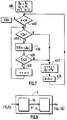
• Figure 7 : un organigramme pour la détermination des enveloppes inférieure et supérieure.
• Figure 8 : un schéma d'un dispositif selon l'invention.
• Figure 9 : un schéma d'un dispositif de codage pour le calcul et le codage d'une droite de régression dans le cas général.
• Figure 10 : un schéma d'un dispositif de codage pour le calcul et le codage d'une droite de régression pour la première variante.
• Figure 11 : un schéma d'un dispositif de transcodage pour le calcul des valeurs de la grandeur dépendante à partir d'un ensemble de droites de régression codées.
• Figure 12 : un schéma d'une réalisation neuronale des moyens de comparaison de la figure 10.
• Figure 13 : une représentation montrant une fonction d'approximation formée de plusieurs droites.
• Figure 14 : deux représentations montrant une détermination des limites de validité de deux droites consécutives.
• Figure 15 : une représentation concernant le raccordement de droites consécutives.

The invention will be better understood using the following figures given by way of non-limiting examples which represent:

• Figure 1: a graph showing a two-dimensional representation of a set of points with a regression line D.
• Figure 2: a graph showing a set of points and lines used to determine an envelope.
• Figure 3: a flowchart of a first variant of implementation of the method from triplets of points.
• Figure 4: a flow diagram of a second variant of implementation of the method from triplets of points.
• Figure 5: part of the flowchart of a third variant of implementation of the method from pairs of points.
• Figure 6: a part of the flowchart indicating a preselection of points belonging to a lower envelope or to an upper envelope of all the points.
• Figure 7: a flowchart for determining the upper and lower envelopes.
• Figure 8: a diagram of a device according to the invention.
• Figure 9: a diagram of a coding device for the calculation and coding of a regression line in the general case.
• Figure 10: a diagram of a coding device for the calculation and coding of a regression line for the first variant.
• Figure 11: a diagram of a transcoding device for calculating the values of the dependent quantity from a set of coded regression lines.
• Figure 12: a diagram of a neural embodiment of the comparison means of Figure 10.
• Figure 13: a representation showing an approximation function formed by several lines.
• Figure 14: two representations showing a determination of the validity limits of two consecutive lines.
• Figure 15: a representation concerning the connection of consecutive straight lines.

The invention relates to the approximation of a known function only through a certain number of points, for example P₁ ... P₆ (Figure 1) in a two-dimensional representation. Each of these points is defined by a pair of values (x, y) connecting the independent quantity x to the dependent quantity y. Thereafter, it will be a question of a pair (respectively of a triplet) of points, which implements two couples (respectively three couples) of values. The points are ordered according to an increasing order of the values of abscissa X _i , which defines an index i increasing with said values. A reverse agreement can be made by modifying the presentation below accordingly.

où x et y sont des variables courantes.According to the invention, an approximation is made of the set of couples (X₁, Y₁), (X₂, Y ...) ... by a regression line D having as equation:

$\text{(1)}\mathit{\text{D}}\text{:}\mathit{\text{y}}\text{=}\mathit{\text{p}}\text{.}\mathit{\text{x}}\text{+}\mathit{\text{q}}\text{.}$

where x and y are common variables.

For this, in a first variant, three pairs of values are considered, for example (X₃, Y₃), (X₄, Y₄), (X₅, Y₅), and a regression line D is determined by balancing the absolute errors. An error is measured by the difference appearing, for a given abscissa x, between the value y of the point and the abscissa y measured on the regression line. Balancing errors on three points, consists of having three equal errors in value absolute with an error sign opposite to the other two for the point having an abscissa x included between the abscissas x of the two other points. Then we examine if for the remaining points of the set, the error which separates them from the line remains less than or equal in absolute value to the error previously determined for the three selected points. This follows from the fact that we are interested in a worst case error relating to the set of all the points to be taken into account, that is to say the largest error, in absolute value, which exists between one of the points and the regression line. If all the errors are effectively less than or equal, the line is selected to represent the points otherwise the operations are repeated with three new pairs of values to determine another regression line.

There can be several regression lines representing all the points of the set. According to the method, the optimal regression line is determined which minimizes the worst case error defined previously.

Figure 1 shows an example formed by six points P₁ to P₆ arranged in a two-dimensional representation. For explanatory purposes consider the final result. It is observed that the regression line D of FIG. 1 is located so that the errors are equal in absolute value for the points P₃, P₄ and P₅. For the points P₁, P₂, P₆ the errors are lower than the previous ones, in absolute value. In a set of points P₁ to P₆, the method will thus consist in seeking the three particular points, here P₃, P₄, P₅, which make it possible to determine the line of optimal regression which minimizes the worst case error then to code this line. In the case of FIG. 1 representing a final result, if two lines D₁ and D₂ are drawn, parallel to the regression line D, which pass respectively through the points P₃, P₅, on the one hand and P₄ on the other hand, we note that all the points of the set are inside a strip limited by the lines D₁ and D₂ or on these lines.

The phase of determining the regression line can give rise to several implementations of which only the most advantageous will be described below.

First variant of the first phase of the method .

FIG. 3 represents the continuation of the steps to be implemented to determine the optimal regression line.

avec

${\text{E}}_{\text{PD}}{\text{(P}}_{\text{i}}{\text{, D) = Y}}_{\text{i}}{\text{- (p.X}}_{\text{i}}\text{+ q)}$

et des relations analogues pour les autres erreurs.Among the set of points P₁ ... P _N (block 100), we select (block 102) any three points P _i , P _j , P _k with i <j <k. These three points are used to determine the regression line which minimizes the error on y for these three points. This determination is preferably carried out analytically by programmed means. A regression line D is determined so that three errors (block 104):
E _PD (P _i , D), E _PD (P _j , D), E _PD (P _k , D)
between the line D and each of the points verify:

${\text{E}}_{\text{PD}}{\text{(P}}_{\text{i}}{\text{, D) = -E}}_{\text{PD}}{\text{(P}}_{\text{j}}{\text{, D) = E}}_{\text{PD}}{\text{(P}}_{\text{k}}\text{, D)}$

with

${\text{E}}_{\text{PD}}{\text{(P}}_{\text{i}}{\text{, D) = Y}}_{\text{i}}{\text{- (pX}}_{\text{i}}\text{+ q)}$

and similar relationships for other errors.

et

   L'erreur se rapportant à un triplet (P_i, P_j, P_k) s'écrit alors :

${\mathit{\text{E}}}_{\mathit{\text{T}}}\text{(}{\mathit{\text{P}}}_{\mathit{\text{i}}}\text{,}{\mathit{\text{P}}}_{\mathit{\text{j}}}\text{,}{\mathit{\text{P}}}_{\mathit{\text{k}}}\text{) = |}{\mathit{\text{E}}}_{\mathit{\text{PD}}}\text{(}{\mathit{\text{P}}}_{\mathit{\text{i}}}\text{,}\mathit{\text{D}}\text{) |}$

   Lorsque l'erreur E_T a été ainsi calculée, on examine si les autres points de l'ensemble engendrent des erreurs inférieures ou égales, en valeur absolue, à celles des points P_i, P_j, P_k. Pour cela on sélectionne un point P_m (bloc 106) additionnel et on calcule la valeur absolue de l'erreur E_Pm (bloc 108) apparaissant entre la valeur de la variable y au point P_m et la droite D.The regression line D is determined using the coefficients p and q of equation (1) such that:

and

The error relating to a triplet (P _i , P _j , P _k ) is then written:

${\mathit{\text{E}}}_{\mathit{\text{T}}}\text{((}{\mathit{\text{P}}}_{\mathit{\text{i}}}\text{,}{\mathit{\text{P}}}_{\mathit{\text{j}}}\text{,}{\mathit{\text{P}}}_{\mathit{\text{k}}}\text{) = |}{\mathit{\text{E}}}_{\mathit{\text{PD}}}\text{((}{\mathit{\text{P}}}_{\mathit{\text{i}}}\text{,}\mathit{\text{D}}\text{) |}$

When the error E _T has been thus calculated, it is examined whether the other points of the set generate errors less than or equal, in absolute value, to those of the points P _i , P _j , P _k . To do this, select an additional point P _m (block 106) and calculate the absolute value of the error E _Pm (block 108) appearing between the value of the variable y at point P _m and the line D.

When this error E _Pm is less than or equal in absolute value to E _T (block 110) (mark Y), the additional point P _m is accepted and the method continues (block 112) with a point following additional (block 106). If all the additional points satisfy the criterion | E _Pm | ≦ E _T , the line D is accepted and its coefficients are used to code the line of optimal regression D _opt (block 114).

When this error E _Pm is greater than E _T (block 110) (mark N), the selected triplet of points P _i , P _j , P _k is not accepted and another triplet of points (block 116) is chosen ( link 101) in the set of points (block 102). The method ends with obtaining the line D (block 114) satisfying this criterion even if all the triplets of points have not been examined.

où α est un coefficient légèrement supérieur à 1. Dans cette même situation, il est également possible de faire appel à la deuxième variante.There may appear situations where, at the end of step 116, all the possible points have been examined and none of the triplets has provided a solution (block 118). In this case, it is possible to resume the sequence of the first variant by replacing the test of block 110 with the following test:

$\text{|}{\mathit{\text{E}}}_{\mathit{\text{Pm}}}\text{| ≦}\mathit{\text{α}}\text{.}{\mathit{\text{E}}}_{\mathit{\text{T}}}$

where α is a coefficient slightly greater than 1. In this same situation, it is also possible to use the second variant.

A -

sélection de trois couples de valeurs parmi ladite suite,

B -

calcul de la fonction linéaire courante de régression D et détermination d'une erreur de triplet ${\mathit{\text{E}}}_{\mathit{\text{T}}}\text{=|}{\mathit{\text{E}}}_{\mathit{\text{PD}}}\text{|}$

s'y rapportant,

C -

sélection d'un couple additionnel,

D -

calcul d'une erreur additionnelle E_Pm entre le couple additionnel et ladite fonction,

E -

et lorsque | E _Pm | ≦ E _T (110) pour le couple additionnel, la méthode reprend à l'étape C avec un couple additionnel suivant,

F -

et lorsque | E _Pm | > E _T pour au moins un couple additionnel,

   la méthode reprend à l'étape A avec une sélection d'un autre groupe de trois couples parmi ladite suite de couples,

G -

et lorsque | E _Pm | ≦ E _T pour tous les couples additionnels, la fonction linéaire courante de régression est codée et stockée en tant que fonction linéaire d'approximation.

The first phase can include the following steps:

AT -

selection of three pairs of values from said sequence,

B -

calculation of the current linear regression function D and determination of a triplet error ${\mathit{\text{E}}}_{\mathit{\text{T}}}\text{= |}{\mathit{\text{E}}}_{\mathit{\text{PD}}}\text{|}$

relating to it,

VS -

selection of an additional couple,

D -

calculation of an additional error E _Pm between the additional torque and said function,

E -

and when | E _Pm | ≦ E _T (110) for the additional torque, the method resumes in step C with a following additional torque,

F -

and when | E _Pm | > E _T for at least one additional torque,

the method resumes in step A with a selection of another group of three couples from said sequence of couples,

G -

and when | E _Pm | ≦ E _T for all additional couples, the current linear regression function is coded and stored as a linear approximation function.

One can choose to scrutinize all the triplets by taking an ascending order or a decreasing order or a random order to carry out this examination. The triplet which will be used to determine the regression line can therefore be detected at any time during the course of this scan. It follows that the speed of obtaining the regression line depends on the instant during which the triplet is detected. Its implementation has a degree of complexity ranging from N to N⁴ where N is the number of initial points. Its complexity is therefore reduced for a small number of points. This variant makes it possible to obtain a material embodiment with strong parallelization. It is very insensitive to a truncation of values and provides an exact result.

Second variant of the first phase of the method.

In this second variant (FIG. 4), we successively select triplets of points, we calculate each time a regression line, and, by induction, we select the one that delivers the largest error E _PD that is say corresponding to the worst case error for the set of points considered.

A -

sélection de trois couples de valeurs parmi ladite suite,

B -

calcul d'une fonction linéaire courante de régression D et détermination d'une erreur de triplet ${\mathit{\text{E}}}_{\mathit{\text{T}}}\text{=|}{\mathit{\text{E}}}_{\mathit{\text{PD}}}\text{|}$

s'y rapportant,

C -

comparaison de l'erreur E_T avec une erreur optimale E_op initialisée à une valeur strictement négative,

D -

et lorsque E _T > E _op , mise à jour de l'erreur optimale E_op en remplaçant E_op par E_T et mise à jour des codes d'une fonction linéaire optimale de régression D_op en remplaçant ceux-ci par les codes de la fonction linéaire courante D,

E -

puis retour à l'étape A pour sélectionner trois autres couples,

F -

et lorsque tous les triplets de couples de valeurs de la suite ont été testés, les derniers codes de la fonction linéaire optimale D_op constituent les codes de la fonction linéaire d'approximation.

According to the second variant, the first phase comprises the following stages:

AT -

selection of three pairs of values from said sequence,

B -

calculation of a current linear regression function D and determination of a triplet error ${\mathit{\text{E}}}_{\mathit{\text{T}}}\text{= |}{\mathit{\text{E}}}_{\mathit{\text{PD}}}\text{|}$

relating to it,

VS -

comparison of the error E _T with an optimal error E _op initialized to a strictly negative value,

D -

and when E _T > E _op , update of the optimal error E _op by replacing E _op by E _T and update of the codes of an optimal linear function of regression D _op by replacing these by the codes of the current linear function D,

E -

then return to step A to select three other couples,

F -

and when all the triples of pairs of values in the sequence have been tested, the last codes of the linear function optimal D _op constitute the codes of the linear approximation function.

On each examination of a triplet, the error E _{T of} said triplet is compared with the optimal error previously stored and the optimal error E _{op is} updated with the largest value of the error E _T determined for each triplet . The parameters of the optimal line are also updated. Before the implementation of step A, the value E _op must be initialized to a negative low value, for example -1.

In this case, the speed of obtaining the regression line does not depend on the mode of scanning the triplets. Its complexity is of degree N³. A hardware implementation can benefit from the great regularity of the algorithm implemented. It is not very sensitive to data truncation and provides an exact solution.

Third variant of the first phase of the method.

A1 -

modifie l'étape A en opérant une sélection de deux couples de valeurs appartenant à ladite suite, tel qu'il existe au moins un couple additionnel intermédiaire ayant une grandeur indépendante (X₁ - X₆) comprise entre les grandeurs indépendantes dudit couple pour constituer au moins un triplet de couples,

A2 -

modifie l'étape A premièrement en déterminant une fonction linéaire annexe qui contient les deux couples sélectionnés et deuxièmement en déterminant des secondes erreurs entre les grandeurs dépendantes des couples intermédiaires possibles et ladite fonction linéaire annexe :

• . et lorsque ces secondes erreurs sont toutes de même signe, sélection du couple intermédiaire fournissant la plus grande seconde erreur, en valeur absolue, pour former un triplet de couples de valeurs formé du couple intermédiaire et des deux couples sélectionnés,
• . et lorsque ces secondes erreurs sont de signes différents, reprise de la méthode à l'étape A1,

B1 -

l'étape B est effectuée avec ledit triplet sélectionné,

C1 -

modifie l'étape C en sélectionnant un couple additionnel dont la grandeur indépendante n'est pas comprise entre la grandeur indépendante des deux couples sélectionnés.

In this third variant (Figure 5), we first select a pair of points to which we add an additional point, located between these two points, to form a triplet of points. For this, the steps A, B and C of the first variant are modified, the other steps remaining the same. The modified steps are such as:

A1 -

modifies step A by operating a selection of two pairs of values belonging to said sequence, such that there is at least one additional intermediate couple having an independent quantity (X₁ - X₆) comprised between the independent quantities of said couple to constitute at least a triplet of couples,

A2 -

modifies step A first by determining a linear annex function which contains the two selected couples and secondly by determining second errors between the quantities dependent on the possible intermediate couples and said linear annex function:

• . and when these second errors are all of the same sign, selection of the intermediate torque providing the largest second error, in absolute value, to form a triplet of pairs of values formed by the intermediate couple and the two selected couples,
• . and when these second errors are of different signs, resumption of the method in step A1,

B1 -

step B is carried out with said triplet selected,

C1 -

modifies step C by selecting an additional couple whose independent quantity is not between the independent quantity of the two selected couples.

When the error | E _Pm | is greater than the error E _T (block 110), the method resumes at step A1 (link 101) with a new selection of pair of points (block 102a).

We observe that the progress of this third variant depends on the scrutiny of the values and therefore of the values themselves. The complexity of the implementation of this variant varies between N and N³ which gives it a certain advantage compared to the previous variants. A strong parallelization of the means of implementation can be carried out but the implementation of the means can present a lack of regularity which can constitute a handicap for an integrated realization. This variant is not very sensitive to rounding errors in values and provides an exact solution.

Fourth variant of the first phase of the method.

It concerns the determination of the regression line from the envelopes.

It is possible to reduce the number of triples to be examined by determining the upper and lower envelopes respectively surrounding the extreme points in the two-dimensional representation of the set of points. An upper envelope or a lower envelope is defined such that by joining any two adjacent points of the envelope with a straight line, all the other points are situated on the same side respectively of the upper envelope or of the lower envelope. All the points belonging to these said envelopes are thus determined.

The determination of the regression line will consist in considering the pairs of adjacent points of one of the envelopes to which an intermediate point not belonging to said envelope is associated to constitute a triplet and to operate like this. has just been described in the case of the pairs of points of the third variant. If an optimal solution has not been found, consider the pairs of points in the other envelope.

To implement an envelope, select a pair of adjacent points belonging to the envelope. It is then determined whether there is a point arranged so that its abscissa is intermediate between the abscissas of the selected points. When this point does not exist, we pass to another pair of points of the same envelope. For certain pairs, when it appears that there are one or more of these intermediate points, the intermediate point furthest from the line containing the two points of the pair is chosen to form a triplet and to determine a regression line. To determine whether this regression line can be selected as the optimal regression line, the method implements the same operations as those described previously in the case of the third variant.

For this, the third variant is modified such that (FIG. 6), prior to step 102a (FIG. 5), the first phase of the method comprises a step (block 100a) of determining a lower envelope and / or of an upper envelope bringing together the most extreme points of the set of points, the selection of the pairs of points in step 102a being made from the adjacent points belonging to one or the other envelope. The selection of said pair of points is carried out when there is at least one intermediate point having an abscissa situated between the abscissas of the points of the pair of points. If there are several intermediate points, the triplet is formed with the intermediate point furthest from the line passing through the two points which form the pair of points. If a solution is not found with the first envelope, the treatment is continued with the second envelope.

The determination of the lower and upper envelopes is carried out according to the flowchart of FIG. 7. The index of the points increasing with the variable x, the first point P _o thus forms part of the two envelopes. Let us first consider the lower envelope, the points belonging to the lower envelope are identified by the letter Q. A current point Q _v is identified by the index v.

et $\text{Q₁ = P₁}$

. Le dernier point courant Q_v est repéré : v = 1 pour P₁. Le nombre k de points traités est comptabilisé.In step 400 the first two points of the envelope are: ${\text{Q}}_{\text{o}}{\text{= P}}_{\text{o}}$

and $\text{Q₁ = P₁}$

. The last current point Q _v is identified: v = 1 for P₁. The number k of points processed is counted.

Step 402: a first test is carried out to determine whether the last point P _N-1 has been processed to detect the end of the determination of the envelope.

Step 404: otherwise we test if v ≧ 1. When v <1 we increment v (v = v + 1) and we take point P _k as point Q _v (step 407). The index k is incremented to process the next point P (step 409) and resumption of the method in step 402.

When v ≧ 1, we calculate a line passing through the points Q _{v - 1} and Q _v (step 406) and we determine the sign ε of the error on the dependent variable between the current point P _k and this line (Q _{v -1} , Q _v ). This is to determine whether the current point is above or below the line (Q _{v - 1} , Q _v ).

When the sign ε ≦ o, we must delete the last point Q _v , decrement v such that v = v - 1 (step 410) and resume the method in step 404. We can in this way be led to delete certain points already accepted when a following point needs to be deleted.

When the sign ε is strictly positive, the method resumes at step 407 with a following point.

This flowchart applies to the determination of the lower and upper envelopes by reversing the sign of the error to be considered.

. On prend P₂ comme deuxième point Q₁. On calcule la droite L_o reliant P₁, P₂. Le segment P₁, P₂ est accepté comme premier segment de l'enveloppe basse. On examine si P₃ est au-dessus de la droite L_o, ce qui est le cas sur la figure 2. Le segment P₂ P₃ est accepté comme deuxième segment de l'enveloppe basse. On calcule ensuite la droite L₁ reliant P₂ et P₃ et on examine si P₄ est au-dessus de la droite L₁. Ce n'est pas le cas sur la figure 2. Ceci entraîne que le point P₃ et la droite L₁ sont d'abord écartés. De même, P₄ est en dessous de la droite L_o donc le point P₂ et la droite L_o sont ensuite aussi écartés comme ne pouvant pas appartenir à l'enveloppe inférieure et les opérations se poursuivent avec la détermination de la droite L₂ reliant P₁, P₄, puis l'examen des points suivants (non représentés).To understand the mechanisms thus implemented, let us consider, by way of example, the simple case formed by the points P₁, P₂, P₃, P₄ of FIG. 2 and determine the lower envelope. The point P₁ is the first point of the envelope from where ${\text{Q}}_{\text{o}}\text{= P₁}$

. We take P₂ as the second point Q₁. We calculate the line L _o connecting P₁, P₂. The segment P₁, P₂ is accepted as the first segment of the lower envelope. We examine if P₃ is above the line L _o , which is the case in Figure 2. The segment P₂ P₃ is accepted as the second segment of the lower envelope. We then calculate the line L₁ connecting P₂ and P₃ and we examine if P₄ is above the line L₁. This is not the case in FIG. 2. This results in the point P₃ and the line L₁ being first discarded. Similarly, P₄ is in below the line L _o therefore the point P₂ and the line L _o are then also discarded as not being able to belong to the lower envelope and the operations continue with the determination of the line L₂ connecting P₁, P₄, then the examination following points (not shown).

The complexity of implementation of this variant based on envelopes is of degree N² and depends on the order of scanning of the data. This complexity is less than that of the previous variants and therefore provides a result quickly. The regularity of the implementation is average but this variant is not very sensitive to rounding errors of the values and delivers an exact solution.

For certain applications, it may be desirable to increase the precision of the determination of the approximation function in certain fields of the independent quantity x and to assign weighting coefficients W _i to the points P _i . This is for example the case when the approximation function is slightly variable with the independent quantity x. Weights can then be assigned to certain points. These can be common to several points or be individual for each point. These weighting coefficients W _i are subsequently considered to be strictly positive.

où E_PD est une valeur signée. La détermination de la droite de régression D pour trois points P_i, P_j, P_k est alors modifiée en ce que les quantités p et q de l'équation (1) deviennent :

$\text{(2) p = NUMP/DET et q = NUMQ/DET}$

où les quantités NUMP, NUMQ et DET sont définies par :

${\text{DET = W}}_{\text{i}}{\text{.W}}_{\text{j}}{\text{.(X}}_{\text{j}}{\text{-X}}_{\text{i}}{\text{) + W}}_{\text{j}}{\text{.W}}_{\text{k}}{\text{.(X}}_{\text{k}}{\text{-X}}_{\text{j}}{\text{) + W}}_{\text{i}}{\text{.W}}_{\text{k}}{\text{.(X}}_{\text{k}}{\text{-X}}_{\text{i}}\text{)}$

${\text{NUMP = W}}_{\text{i}}{\text{.W}}_{\text{j}}{\text{.(Y}}_{\text{j}}{\text{-Y}}_{\text{i}}{\text{) + W}}_{\text{j}}{\text{.W}}_{\text{k}}{\text{.(Y}}_{\text{k}}{\text{-Y}}_{\text{j}}{\text{) + W}}_{\text{i}}{\text{.W}}_{\text{k}}{\text{.(Y}}_{\text{k}}{\text{-Y}}_{\text{i}}\text{)}$

${\text{NUMQ = W}}_{\text{i}}{\text{.W}}_{\text{j}}{\text{.(X}}_{\text{j}}{\text{.Y}}_{\text{i}}{\text{-X}}_{\text{i}}{\text{.Y}}_{\text{j}}{\text{) + W}}_{\text{j}}{\text{.W}}_{\text{k}}{\text{.(X}}_{\text{k}}{\text{.Y}}_{\text{j}}{\text{-X}}_{\text{j}}{\text{.Y}}_{\text{k}}{\text{) + W}}_{\text{i}}{\text{.W}}_{\text{k}}{\text{.(X}}_{\text{k}}{\text{.Y}}_{\text{i}}{\text{-X}}_{\text{i}}{\text{.Y}}_{\text{k}}\text{)}$

   Par ailleurs, l'erreur E_T associée à ce triplet peut être exprimée et calculée par :
avec

${\mathit{\text{E}}}_{\mathit{\text{T}}}\text{(}{\mathit{\text{P}}}_{\mathit{\text{i}}}\text{,}{\mathit{\text{P}}}_{\mathit{\text{j}}}\text{,}{\mathit{\text{P}}}_{\mathit{\text{k}}}\text{) = |}{\mathit{\text{E}}}_{\mathit{\text{PD}}}\text{(}{\mathit{\text{P}}}_{\mathit{\text{i}}}\text{,}\mathit{\text{D}}\text{|}$

${\mathit{\text{E}}}_{\mathit{\text{PD}}}\text{(}{\mathit{\text{P}}}_{\mathit{\text{i}}}\text{,}\mathit{\text{D}}\text{) = -}{\mathit{\text{E}}}_{\mathit{\text{PD}}}\text{(}{\mathit{\text{P}}}_{\mathit{\text{j}}}\text{,}\mathit{\text{D}}\text{) =}{\mathit{\text{E}}}_{\mathit{\text{PD}}}\text{(}{\mathit{\text{P}}}_{\mathit{\text{k}}}\text{,}\mathit{\text{D}}\text{)}$

ou

   La première et la seconde variante de la méthode de la première phase décrites précédemment peuvent être mises en oeuvre en faisant intervenir les coefficients de pondération ci-dessus. Cette mise en oeuvre peut être effectuée en programmant un calculateur.In the cases where weighting coefficients exist, an error E _PD is defined between a point P _i and the regression line D such that:

${\mathit{\text{E}}}_{\mathit{\text{PD}}}\text{((}{\mathit{\text{P}}}_{\mathit{\text{i}}}\text{,}\mathit{\text{D}}\text{) =}{\mathit{\text{W}}}_{\mathit{\text{i}}}\text{. [}{\mathit{\text{Y}}}_{\mathit{\text{i}}}\text{- (}\mathit{\text{p}}\text{.}{\mathit{\text{X}}}_{\mathit{\text{i}}}\text{+}\mathit{\text{q}}\text{)]}$

where E _PD is a signed value. The determination of the regression line D for three points P _i , P _j , P _k is then modified in that the quantities p and q of equation (1) become:

$\text{(2) p = NUMP / DET and q = NUMQ / DET}$

where the quantities NUMP, NUMQ and DET are defined by:

${\text{DET = W}}_{\text{i}}{\text{.W}}_{\text{j}}{\text{. (X}}_{\text{j}}{\text{-X}}_{\text{i}}{\text{) + W}}_{\text{j}}{\text{.W}}_{\text{k}}{\text{. (X}}_{\text{k}}{\text{-X}}_{\text{j}}{\text{) + W}}_{\text{i}}{\text{.W}}_{\text{k}}{\text{. (X}}_{\text{k}}{\text{-X}}_{\text{i}}\text{)}$

${\text{NUMP = W}}_{\text{i}}{\text{.W}}_{\text{j}}{\text{. (Y}}_{\text{j}}{\text{-Y}}_{\text{i}}{\text{) + W}}_{\text{j}}{\text{.W}}_{\text{k}}{\text{. (Y}}_{\text{k}}{\text{-Y}}_{\text{j}}{\text{) + W}}_{\text{i}}{\text{.W}}_{\text{k}}{\text{. (Y}}_{\text{k}}{\text{-Y}}_{\text{i}}\text{)}$

${\text{NUMQ = W}}_{\text{i}}{\text{.W}}_{\text{j}}{\text{. (X}}_{\text{j}}{\text{.Y}}_{\text{i}}{\text{-X}}_{\text{i}}{\text{.Y}}_{\text{j}}{\text{) + W}}_{\text{j}}{\text{.W}}_{\text{k}}{\text{. (X}}_{\text{k}}{\text{.Y}}_{\text{j}}{\text{-X}}_{\text{j}}{\text{.Y}}_{\text{k}}{\text{) + W}}_{\text{i}}{\text{.W}}_{\text{k}}{\text{. (X}}_{\text{k}}{\text{.Y}}_{\text{i}}{\text{-X}}_{\text{i}}{\text{.Y}}_{\text{k}}\text{)}$

Furthermore, the error E _T associated with this triplet can be expressed and calculated by:
with

${\mathit{\text{E}}}_{\mathit{\text{T}}}\text{((}{\mathit{\text{P}}}_{\mathit{\text{i}}}\text{,}{\mathit{\text{P}}}_{\mathit{\text{j}}}\text{,}{\mathit{\text{P}}}_{\mathit{\text{k}}}\text{) = |}{\mathit{\text{E}}}_{\mathit{\text{PD}}}\text{((}{\mathit{\text{P}}}_{\mathit{\text{i}}}\text{,}\mathit{\text{D}}\text{|}$

${\mathit{\text{E}}}_{\mathit{\text{PD}}}\text{((}{\mathit{\text{P}}}_{\mathit{\text{i}}}\text{,}\mathit{\text{D}}\text{) = -}{\mathit{\text{E}}}_{\mathit{\text{PD}}}\text{((}{\mathit{\text{P}}}_{\mathit{\text{j}}}\text{,}\mathit{\text{D}}\text{) =}{\mathit{\text{E}}}_{\mathit{\text{PD}}}\text{((}{\mathit{\text{P}}}_{\mathit{\text{k}}}\text{,}\mathit{\text{D}}\text{)}$

or

The first and the second variant of the method of the first phase described above can be implemented by using the above weighting coefficients. This implementation can be carried out by programming a computer.

In the case where a pair of points is selected by using weighting coefficients W, the method presents the following arrangements.

   Ce facteur F_l intervient dans la détermination du point intermédiaire P_l qui sera à sélectionner (i < l < k) pour constituer le triplet en tenant compte des poids affectant les points. On choisit un point P₁ et on calcule la droite de régression D₁ associée au triplet P_i, P_l, P_k et l'erreur E_Tl associée au triplet.For the points P _i , P _l , P _k which form the triplet, a factor F _l is defined which links the respective coordinates and the respective weighting coefficients of the points P _i , P _l , P _k . At the central point 1, we associate the factor F _l such that:

This factor F _l intervenes in the determination of the intermediate point P _l which will be to be selected (i <l <k) to constitute the triplet taking into account the weights affecting the points. We choose a point P₁ and we calculate the regression line D₁ associated with the triplet P _i , P _l , P _k and the error E _Tl associated with the triplet.

• . d'une part les quantités E_PD (P_i, D_p) pour tous les points intermédiaires,
• . d'autre part les quantités (a) suivantes, uniquement pour les points intermédiaires pour lesquels F_l < 1 avec
  

   S'il existe au moins un point intermédiaire tel que F_l > 1, on définit également une grandeur G_min qui est la valeur minimale prise par (a) uniquement pour les points intermédiaires tels que F_l > 1. On examine alors s'il existe au moins un point intermédiaire tel que :
   E_PD (P_i, D_l) ≧ 0
   G_max ≦ α E_Tl
   et G_min. α ≧ E_Tl (α, coefficient ≧ 1). S'il existe un tel point, il est choisi comme point intermédiaire pour former le triplet.This variant of the method consists in modifying only step A2 of the third variant (block 102b, FIG. 5). This step determines the existence and the value of an intermediate point used to form a triplet. We first try to form a regression line located below P _i and P _k . For each intermediate point P _l , we determine if F _l = 1 and E _PD (P _i , D _l ) <0. If at least one point satisfies this condition, there is no regression line located below P _i and P _k , otherwise we determine a quantity G _max which is the maximum quantity among:

• . on the one hand, the quantities E _PD (P _i , D _p ) for all intermediate points,
• . on the other hand the following quantities (a), only for the intermediate points for which F _l <1 with
  

If there is at least one intermediate point such as F _l > 1, we also define a quantity G _min which is the minimum value taken by (a) only for the intermediate points such as F _l > 1. We then examine s' there is at least one intermediate point such as:
E _PD (P _i , D _l ) ≧ 0
G _max ≦ α E _Tl
and G _min . α ≧ E _Tl (α, coefficient ≧ 1). If there is such a point, it is chosen as an intermediate point to form the triplet.

If there is no intermediate point such as F₁> 1, we test if there is at least one intermediate point such that:
E _PD (P _i , D _l ) ≧ 0
G _max ≦ α.E _Tl (α: coefficient ≧ 1).

If such a point exists, it is chosen as an intermediate point to form the triplet.

If no triplet has been formed, we seek to form a regression line located above the points P _i and P _k . The same method is repeated by reversing the sign of the errors E _PD .

If no point P _l can be selected, we start again with another pair P _i , P _k .

When the set of points to be treated is too large to be represented by a single regression line, the method then codes several regression lines each being determined according to the method described above.

Figure 13 shows an example in which the approximation function consists of several regression lines.

In a first situation, by knowing the quantities to be treated, we may want to impose limits on each regression line according to the independent quantity x. So we may want to have a regression line D _a between the values [ X _a , X _b [of the quantity, bound x _a included, bound x _b excluded. Likewise with D _b for [ X _b , X _c [and D _c for [ X _c , X _d [. In this case the problem amounts to determining a line in a limited domain and to applying each time the method already described.

But it is possible to make that for each line, the method determines limits according to the independent quantity x without them being fixed at the start.

, où N est le nombre total de points. Les droites D1 et D2 forment une approximation avec respectivement des erreurs maximales E1 et E2. Supposons que E2 soit supérieure à E1 et que l'on cherche à réduire E2, il faut alors transférer vers D1 un point appartenant à D2. Lorsque le nombre de points diminue, l'erreur résultante est soit inchangée soit réduite. Lorsque le nombre de points augmente, l'erreur résultante est soit inchangée soit augmentée. En fonction du nombre n de points appartenant aux droites D1 et D2, les variations des erreurs E1 et E2 peuvent présenter les allures représentées sur la figure 14-B pour l'exemple choisi. Il s'ensuit que l'approximation obtenue globalement par D1 et D2 est optimale lorsque ces erreurs sont voisines, c'est-à-dire situées dans la zone délimitée par un trait discontinu sur la figure 14-B. Ces erreurs ne sont pas nécessairement égales compte tenu du caractère discontinu des valeurs de la grandeur indépendante.The principle of the determination of an optimal limit between two adjacent regression lines is represented on the figure 14-A. Let there be two non-optimal regression lines D1 and D2. The line D1 is determined from N1 points and the line D2 is determined from the remaining N2 points with $\text{N1 + N2 = N}$

, where N is the total number of points. The lines D1 and D2 form an approximation with respectively maximum errors E1 and E2. Suppose that E2 is greater than E1 and that we seek to reduce E2, we must then transfer to D1 a point belonging to D2. When the number of points decreases, the resulting error is either unchanged or reduced. When the number of points increases, the resulting error is either unchanged or increased. Depending on the number n of points belonging to the lines D1 and D2, the variations of the errors E1 and E2 can present the paces represented on the figure 14-B for the chosen example. It follows that the approximation obtained globally by D1 and D2 is optimal when these errors are close, that is to say located in the zone delimited by a broken line on the figure 14-B. These errors are not necessarily equal given the discontinuous nature of the values of the independent quantity.

• on détermine la droite D1 sur un certain nombre de points et on calcule l'erreur E1 maximale,
• on détermine la droite D2 sur les points restants et on calcule l'erreur E2 maximale,
• on compare E1 et E2 et on transfère un point de la droite qui présente la plus forte erreur vers la droite qui présente la plus faible erreur,
• on détermine la valeur limite X_lim lorsqu'il se produit une inversion dans le rapport entre les deux erreurs.

To determine the value of abscissa X _lim between the two lines:

• the line D1 is determined on a certain number of points and the maximum error E1 is calculated,
• the line D2 is determined on the remaining points and the maximum error E2 is calculated,
• we compare E1 and E2 and we transfer a point from the line which presents the greatest error to the line which presents the smallest error,
• the limit value X _lim is determined when an inversion in the relationship between the two errors occurs.

This method applies by induction to several lines delimited between them by several abscissa limits.

The lines are determined from a discrete and limited series of measured variables. However, for the exploitation of regression lines, it is necessary to define their domain of existence which extends over a continuum of values located between two abscissa limits. Now the determination of the lines provides a series of lines which do not necessarily connect by their ends. It may appear useful for certain applications to avoid a difference appearing on the value of the dependent quantity y for values close to (X _lim - ε) and (X _lim + ε) of the independent quantity where ε is a very small value. It is possible to choose that the limit abscissa X _lim belongs exclusively to one or the other line. It is also possible to follow the determination of the right-hand sequences of a procedure for connecting lines.

This is shown in FIG. 15. One solution may consist in validating the line D1 up to the abscissa of the first point belonging to the line D2 and in recalculating the line D2 from the new value of dependent quantity y thus determined. By keeping the last point belonging to D2, a new line D'2 is thus represented, shown in dotted lines in FIG. 15. A similar procedure can be applied to substitute the line D'3 for the line D3. We thus obtain an assembly formed by several regression lines formed, in the example described, by lines D1, D'2, D'3. This set constitutes an approximation of the measured quantities by reducing a maximum error between the measured quantities and the set of lines. A variant more suited to this reduction consists in making it the lines corresponding to the largest errors which impose their limit points as limit points to the lines corresponding to weaker errors.

Device for implementing the first phase

A diagram of a device for generating an approximation function according to the invention is shown in Figure 8. The device 5 receives couples (X _i , Y _i ) associating the dependent quantity Y _i with the independent quantity X _i . The pairs (X _i , Y _i ) enter the first means 10 to determine and code the linear regression function forming an approximation of the measurement pairs. The specific codes thus determined are transmitted (connection 9) to the second means 17 which determine second pairs (X _A , Y ′ _A ) according to the codes specific to the approximation function.

We distinguish on the one hand the second variant which determines all the regression lines passing through each feasible combination of triplets with the sequence of first couples, and the other variants for which each regression line determined (associated with its error E _T ) , we examine whether the remaining additional points do indeed provide additional errors less than or equal to the triplet error E _T.

• une mémoire 12c MEM qui stocke notamment tous les points appartenant à l'ensemble de points à traiter. Ces points sont représentés par leurs coordonnées (x, y), et éventuellement leurs poids W ou leurs inverses 1/W,
• une unité de calcul 13c COMPUT qui calcule, pour chaque triplet sélectionné, la droite de régression adaptée à chaque triplet, c'est-à-dire les codes p, q de la droite et l'erreur E_T associée au triplet.

FIG. 9 represents a device adapted to the second variant. He understands :

• a memory 12c MEM which stores in particular all the points belonging to the set of points to be processed. These points are represented by their coordinates (x, y), and possibly their weights W or their inverses 1 / W,
• a computation unit 13c COMPUT which calculates, for each triplet selected, the regression line adapted to each triplet, that is to say the codes p, q of the line and the error E _T associated with the triplet.

In addition, a controller 11c CONTR makes it possible to carry out the management of the operations and to address new triplets by carrying out the reads / writes of the memory 12c and the loading of the computing unit 13c by new triplets. The selection of the regression line which is to be kept, that is to say for this variant that delivering the largest triplet error, is carried out by the calculation unit 13c.

FIG. 10 corresponds to the case of the other variants for which, for each current regression line, it is examined whether the other additional points of the sequence deliver an error lower than the triplet error.

For this, the first means 10 comprise a unit 13c calculation and a comparison unit 14c forming calculation means 19c.

Si la droite de régression courante n'est pas acceptée (test positif), un autre triplet est sélectionné et une procédure analogue est à nouveau effectuée. Si le test est négatif pour tous les points additionnels, la droite de régression est acceptée et ses paramètres sont chargés par l'unité de calcul 13c dans la mémoire 12c.The calculation unit 13c transmits the codes p, q of the regression line of the current triplet to the comparison unit 14c COMPAR which determines whether the additional points of the set of points generate a weaker error with this line of regression than that generated by the points of the current triplet. For this, the comparison unit 14c performs the test:

$\text{|}{\mathit{\text{E}}}_{\mathit{\text{Pm}}}\text{| >}{\mathit{\text{E}}}_{\mathit{\text{T}}}$

If the current regression line is not accepted (positive test), another triplet is selected and a similar procedure is performed again. If the test is negative for all the additional points, the regression line is accepted and its parameters are loaded by the calculation unit 13c into the memory 12c.

For the variants which operate from a pair of points, the calculation unit 13c is programmed to determine the intermediate points and to form the triplets coming from the pairs of points, these being themselves possibly coming from envelopes of points. In the latter case, the calculation unit 13c is also programmed to determine the envelopes. The comparison unit 14c then performs the comparisons of the errors relating to the different triples.

• les lectures/écritures de la mémoire 12c,
• le chargement de l'unité de calcul 13c par de nouveaux triplets,
• l'appel vers l'unité de comparaison 14c de tous les points additionnels à examiner successivement.

To manage operations and send new triplets (when triplets examined have not been satisfactory), the device includes, as before, a controller 11c which manages:

• reads / writes from memory 12c,
• loading of the calculation unit 13c with new triples,
• the call to the comparison unit 14c of all the additional points to be examined successively.

It is possible to implement the first phase of the method using comparison means 14c (FIG. 12) having a neural structure. Let us consider the most complete case where there are weighting coefficients associated with each point P _i . When these coefficients do not exist, it suffices to give them a unit value in the following explanations. By way of example, it is possible to store in the memory 12c (FIGS. 9, 10) the inverses of the coefficients W _i individually assigned to the points P _i . The calculation unit 13c determines according to equations (2) and (3), for a given triplet, the codes: -p, -q, E _T and - E _T.

ou

${\text{Y}}_{\text{m}}{\text{- p.X}}_{\text{m}}{\text{+ (E}}_{\text{T}}{\text{/W}}_{\text{m}}\text{) - q < 0.}$

The condition to be tested in unit 14c for an additional point P _m to be tested, of parameters X _m , Y _m , W _m , is:

${\text{Y}}_{\text{m}}{\text{- pX}}_{\text{m}}{\text{- (E}}_{\text{T}}{\text{/ W}}_{\text{m}}\text{) - q> 0}$

or

${\text{Y}}_{\text{m}}{\text{- pX}}_{\text{m}}{\text{+ (E}}_{\text{T}}{\text{/ W}}_{\text{m}}\text{) - q <0.}$

These tests are easily carried out by a unit 14c having a neural organization. Indeed, this test is made up of linear functions, thresholding functions and logical functions easily performed in a neural network.

Such a neural comparison unit is represented in FIG. 12. It comprises three neurons N1, N2, N3. Neurons N1 and N2 receive data E1, E2, E3, E4. Neuron N3 receives the outputs of neurons N1 and N2. Each of the inputs of these neurons is assigned a synaptic coefficient Ci according to the known technique implemented in neural networks. This technique is for example described in R.P. LIPPMANN, "An introduction to computing with neural nets" IEEE ASSP Magazine, April 1987, pp. 4 to 22.

To carry out the preceding tests, the neurons N1 and N2 are programmed according to Table I: TABLE I Neuron E₁ C₁ E₂ C₂ E₃ C₃ E₄ C₄ 1 Y _m 1 X _m - p 1 / W _m - E _T 1 - q 2 Y _m 1 X _m - p 1 / W _m E _T 1 - q

All the synaptic coefficients of neuron N3 are equal to 1.

   A ce potentiel s, il faut appliquer une fonction d'activation A. Pour les neurones N1 et N3, la fonction d'activation A₁ est :

$\text{A₁(s) = 1 si s > 0}$

$\text{A₁(s) = 0 si s ≦ 0.}$

The neurons N1 and N2 each calculate a neuronal potential s such that: $\mathit{\text{s}}\text{=}{\mathit{\text{Σ}}}_{\mathit{\text{i}}}{\mathit{\text{VS}}}_{\mathit{\text{i}}}\text{.}{\mathit{\text{E}}}_{\mathit{\text{i}}}$

To this potential s, it is necessary to apply an activation function A. For the neurons N1 and N3, the activation function A₁ is:

$\text{A₁ (s) = 1 if s> 0}$

$\text{A₁ (s) = 0 if s ≦ 0.}$

For neuron N2, the activation function A₂ is:

A₂ (s) = 1 if s <0

$\text{A₂ (s) = 0 if s ≧ 0.}$

The output of neuron N3 is worth 1 if the condition to be tested is satisfied and is worth 0 in the opposite case.

We observe in table I that the data -p, -q, -E _T , + E _T are codes which appear as synaptic coefficients in the diagram of FIG. 12. The data Y _m , X _m , 1 / W _m are data which appear on the entries of the same diagram. When all the additional points have been tested and a regression line has been selected, the codes p, q, W loaded into the memory 12c are then used to implement the second phase of the method (FIG. 11).

The advantage presented by the neural realization described is to be able to parallelize the different operations to be implemented according to the variants already described. The operation of such a neural realization is then very rapid.

When the regression lines have been determined, the second phase consisting in calculating second pairs (X _A , Y ′ _A ) of values of the quantities is then implemented in decoding means 17 (FIG. 11). The codes of the lines are loaded into a memory 12a which during the second phase is addressed, by a controller 11a, to supply the codes of the regression lines addressed. The memory 12a, organized in lines for example, contains for each regression line the parameters p, q and x _L where x _L is the upper abscissa limit for which each regression line is defined.

correspondant aux m droites de régression stockées.The memory 12a thus contains an array of parameters

corresponding to the m regression lines stored.

• le contrôleur 11_a,
• la mémoire 12_a,
• et une unité de décodage 13_a. Celle-ci reçoit une valeur de requête X_A de la grandeur indépendante pour laquelle on désire obtenir un résultat Y'_A issu de la fonction d'approximation. Pour cela le contrôleur 11_a présente successivement certaines lignes de codes de la mémoire 12_a et, pour chaque ligne de codes, l'unité de décodage 13_a teste le code x_L pour déterminer si la valeur X_A de la grandeur d'entrée peut être traitée par la droite de régression codée par ladite ligne. Si cela n'est pas le cas, l'unité 13_a requiert du contrôleur 11_a une autre ligne de codes. Lorsque cette condition est vérifiée, l'unité 13_a effectue le calcul :
  
  ${\text{Y'}}_{\text{A}}{\text{= p}}_{\text{n}}{\text{.X}}_{\text{A}}{\text{+ q}}_{\text{n}}$
  
  
  
  si la ligne d'ordre n est la ligne adéquate.

The decoding means 17 include:

• the controller 11 _has,
• the memory _12a,
• and a decoding unit 13 _a . This receives a request value X _A of the independent quantity for which one wishes to obtain a result Y ' _A from the approximation function. For this, the controller 11 _a successively presents certain lines of codes of the memory 12 _a and, for each line of codes, the decoding unit 13 _a tests the code x _L to determine whether the value X _A of the input quantity can be processed by the regression line coded by said line. If this is not the case, the unit _has 13 requires the controller 11 _has another line of code. When this condition is verified, the unit 13 _a calculates:
  
  ${\text{Y '}}_{\text{AT}}{\text{= p}}_{\text{not}}{\text{.X}}_{\text{AT}}{\text{+ q}}_{\text{not}}$
  
  
  
  if the order line n is the correct line.

• il peut s'agir d'une mémoire 12 unique qui peut stocker les paramètres des couples de valeurs et les codes des droites de régression déterminées. Les unités 12a et 12c forment alors la mémoire 12,
• il peut s'agir d'un contrôleur 11 unique qui regroupe les fonctions des contrôleurs 11c et 11a,
• l'unité de calcul 13c et l'unité de décodage 13a peuvent également former une seule unité 13.

As has just been described, the first means 10 can constitute a coding device and the second means 17 can constitute a decoding device, the two devices being separate. They can indeed be distant from each other, the coding operations being separate from the decoding operations. However, the two means 10 and 17 can also form a single coding / decoding device. In this case, certain organs can be assigned successively to several operations. Especially :

• it may be a single memory 12 which can store the parameters of the pairs of values and the codes of the determined regression lines. The units 12a and 12c then form the memory 12,
• it may be a single controller 11 which combines the functions of the controllers 11c and 11a,
• the calculation unit 13c and the decoding unit 13a can also form a single unit 13.

It is also possible to produce the decoding means 17 (FIG. 11) according to an organization with a parallel structure. One solution then consists in comparing, in parallel, the query quantity X _A with all the codes x _L. We obtain a set of signals T _L representing the results of these comparison tests. One carries out then, in parallel, for all the values of L, a test which combines two by two the signals T _L and T _{L + 1} and which indicates if the quantity of request X _A is in the interval index L. This test is verified for a single value of L, noted n. We then access the corresponding codes p _n and q _n , and we deduce the magnitude Y ' _A in the same way as above.

The first means 10 (coding) associated with the second means 17 (decoding) can be used to determine the value of an approximation function by at least one regression line. These determinations can be carried out for any values of the independent quantity (within predefined limits defining the extent of the action of each regression line). This method avoids unnecessarily storing tables of values, for which all the values will not be used. According to the method, only the values necessary for the application are determined. The method according to the invention has the advantage of only calculating the necessary values. The device of the invention can be used in combination with a neural processor to calculate an approximation of a non-linear function, for example a sigmoid function. A neural processor calculates neural potentials derived from sums of products of synaptic coefficients by states of neurons. The technique is developed in the document by R.P. LIPPMANN already cited. Each neural potential must be subjected to the action of a nonlinear function. For this, each neural potential constitutes the independent quantity described above and the calculation of the function th (x) for example is performed for the only useful query values. The method provides approximate values, but this approximation can be obtained with a precision which can be increased according to the number of regression lines calculated and possibly the weighting coefficients W. The precision remains nevertheless dependent on the precision of the coordinates of the starting couples .

Such a method is particularly interesting for the calculations of known functions (such as mathematical functions) or of explicitly unknown functions, for example a function represented by measurement points, which one wishes to simplify by a linear regression function.

In its neural version, the invention is interesting in neural applications because it not only provides a homogeneous treatment but also great compactness of the necessary hardware architecture.

• . Dans la première combinaison, on utilise tout d'abord la première variante basée sur des triplets de points. Si une solution n'est pas trouvée, on enchaîne avec la deuxième variante basée aussi sur des triplets de points. Ceci permet d'obtenir les avantages suivants :
  • . Quelles que soient les données, on obtient une solution.
  • . Dans le cas où on exige qu'on obtienne toujours une solution exacte, cette combinaison permet d'obtenir la rapidité maximale. En effet, dans le cas général la solution est fournie directement par la première variante appelée, qui est celle fournissant le plus rapidement une solution exacte dans le cas où les poids existent. La deuxième variante est beaucoup plus lente mais elle permet de garantir que la combinaison fournit toujours une solution.
• . Dans la deuxième combinaison, on utilise tout d'abord la variante basée sur des paires de points. Si elle ne trouve pas une solution (qui peut être approchée), on utilise la deuxième variante basée sur des triplets de points. Ceci permet d'obtenir les avantages suivants :
  • . Quelles que soient les données, on obtient une solution (éventuellement approchée).
  • . Cette combinaison est en moyenne plus rapide que la précédente.
  • . En contrepartie, elle ne fournit généralement qu'une solution approchée.

It is possible to combine the variants of the method, in their hardware implementations to combine their advantages. For example, the following combinations are advantageous:
If the weights exist, two combinations appear interesting:

• . In the first combination, we first use the first variant based on triplets of points. If a solution is not found, we continue with the second variant also based on triplets of points. This provides the following advantages:
  • . Whatever the data, we get a solution.
  • . In the case where we demand that we always obtain an exact solution, this combination makes it possible to obtain maximum speed. In fact, in the general case, the solution is provided directly by the first variant called, which is the one that most quickly provides an exact solution in the case where the weights exist. The second variant is much slower, but it ensures that the combination always provides a solution.
• . In the second combination, we first use the variant based on pairs of points. If it does not find a solution (which can be approximated), we use the second variant based on triplets of points. This provides the following advantages:
  • . Whatever the data, we get a solution (possibly approximate).
  • . This combination is on average faster than the previous one.
  • . In return, it generally only provides an approximate solution.

• . Quelles que soient les données, on obtient une solution,
• . Cette combinaison permet d'obtenir la meilleure rapidité moyenne.

In the case where the weights do not exist, an interesting combination consists in first using the variant based on the envelope of the points. If it does not find a solution, we use the second variant based on triplets of points. This provides the following advantages:

• . Whatever the data, we get a solution,
• . This combination provides the best average speed.

When the linear regression function has been determined according to the method described, it is possible to determine not only magnitudes Y ' _A pertaining to said function but also magnitudes resulting from the derivative of said function. Indeed, for a request value X _A of the independent quantity, it suffices to extract from the storage means the value p coming out at the value X _A to know the value of this corresponding derivative.

Claims (12)

Device (5) for generating an approximation function based on first pairs ((X₁, Y₁) to (X₆, Y₆)) of values associating a dependent quantity (Y₁ to Y₆) with an independent quantity (X₁ to X₆), and to determine second pairs (X _A , Y ' _A ) of values of said quantities according to said approximation function characterized in that the device comprises: - first means (10): - to determine iteratively at least one current linear regression function by making equal, in absolute value, first errors, of alternating signs, measured between first values (Y₃, Y₄, Y₅) of the dependent quantity for three couples (X₃, Y₃) (X₄, Y₄) (X₅, Y₅) of a sequence of said first couples, and respectively of the second values (Y'₃, Y'₄, Y'₅) of the dependent quantity determined, according to said linear function current, for the same values (X₃, X₄, X₅) of the independent quantity, - to select that of the current linear functions which delivers the approximation of all the couples of said sequence with minimal errors, - and to code, using specific codes (p, q), the selected linear regression function, - And second means (17) for determining said second couples (X _A , Y ' _A ) using said specific codes. Device according to claim 1 characterized in that the first means (10) comprise: - means (12c) for memorizing the quantities of the first pairs and said specific codes, means (13c) (19c) for successively calculating the specific codes (p, q) of current linear regression functions and their first errors, equalized in absolute value, respective (E _T ) and for selecting at least one current linear function regression, - And means (11c) for controlling the means (12c) for storing and the means (13c) for calculating. Device (5) according to claims 1 or 2 characterized in that to select said linear function, the first means comprise means (14c): to similarly determine additional errors for the other pairs (X₁, Y₁) (X₂, Y₂) (X₆, Y₆) of values of said sequence, - to compare the additional errors with said first equalized errors (E _T ), - And to select the current linear function which provides additional errors less than or equal in absolute value to said first equalized errors (E _T ). Device according to Claim 2, characterized in that, to select the linear regression function, the means for calculating (13c) select that of the current linear regression functions which delivers the first maximum equalized errors (E _T ). Device according to one of Claims 1 to 4, characterized in that the second means (17) comprise: - means (12a) for storing said specific codes of at least one linear regression function, - Means (13a) for selecting, on request of an independent magnitude value (X _A ), a linear regression function coming out at said value, and for calculating, from specific codes received from the means for memorizing, a value of dependent quantity (Y ' _A ) associated with the value of independent quantity (X _A ), - And means (11a) for addressing to the means for calculating, and at their request, the specific codes of the linear regression functions. In a device for generating an approximation function based on first pairs ((X₁, Y₁) - (X₆, Y₆)) of values associating a dependent quantity (Y₁ - Y₆) with an independent quantity (X₁ - X₆), method to generate said approximation function from the first pairs (X₁, Y₁) (X₆, Y₆) of values, and to determine second pairs (X _A , Y ' _A ) of values of said quantities according to said function of approximation, characterized in that, the method comprises: - a first phase: - to iteratively determine at least one current linear regression function by making equal, in absolute value, the first errors E _PD , of alternating signs, measured between the first values (Y₃, Y₄, Y₅) of the dependent quantity for three couples ( X₃, Y₃), (X₄, Y₄) (X₅, Y₅) of a sequence of said first couples, and respectively of the second values (Y'₃, Y'₄, Y'₅) of the dependent quantity determined, according to said linear function, for the same values (X₃, X₄, X₅) of the independent quantity, - to select that of the current linear functions which delivers the approximation of all the couples of said sequence with minimal errors, - and to code the linear regression function selected using specific codes, - And a second phase to determine said second couples (X _A , Y ' _A ) using said specific codes. Method according to claim 6 characterized in that the first phase comprises the following steps: A - selection (102) of three pairs (P3, P4, P5) of values from said sequence, B - calculation (104) of the current linear regression function D and determination of a triplet error ${\mathit{\text{E}}}_{\mathit{\text{T}}}\text{= |}{\mathit{\text{E}}}_{\mathit{\text{PD}}}\text{|}$

relating to it, C - selection (106) of an additional torque (P1), (P2), (P6), D - calculation (108) of an additional error E _Pm between the additional torque and said function, E - and when | E _Pm | ≦ E _T (110) for the additional torque, the method resumes in step C with a following additional torque, F - and when | E _Pm | > E _T for at least one additional couple (110), the method resumes in step A with a selection of another group of three couples from said sequence of couples, G - and when | E _Pm | ≦ E _T for all additional couples (112), the current linear regression function is coded and stored (114) as a linear approximation function. Method according to claim 6 characterized in that the first phase comprises the following steps: A - selection (102) of three pairs (P3, P4, P5) of values from said sequence, B - calculation (104) of a current linear regression function D and determination of a triplet error ${\mathit{\text{E}}}_{\mathit{\text{T}}}\text{= |}{\mathit{\text{E}}}_{\mathit{\text{PD}}}\text{|}$

relating to it, C - comparison (210) of the error E _T with an optimal error E _op initialized to a strictly negative value, D - and when E _T > E _op , updating (114) of the optimal error E _op by replacing E _op by E _T and updating the codes of an optimal linear regression function D _op by replacing those ci by the codes of the current linear function (D), E - then return (116) to step A to select three other couples (102), F - and when all the triplets of pairs of values in the sequence have been tested (116), the last codes of the optimal linear function D _op constitute the codes of the linear approximation function (114). Method according to claim 8 characterized in that the first phase comprises the following modified steps: A1 - modifies step A by making a selection (102a) of two pairs of values belonging to said sequence, such that there is at least one additional intermediate couple having an independent quantity (X₁ - X₆) between the quantities independent of said pair to constitute at least a triplet of pairs of values, A2 - modifies step A first by determining (102b) an additional linear function which contains the two selected couples and secondly by determining second errors between the quantities dependent on the possible intermediate couples and said additional linear function: . and when these second errors are all of the same sign, selection of the intermediate torque providing the largest second error, in absolute value, to form a triplet of pairs of values formed by the intermediate couple and the two selected couples, . and when these second errors are of different signs, resumption of the method in step A1, B1 - step B (104) is carried out with said selected triplet, C1 - modifies step C (106) by selecting (106a) an additional couple whose independent quantity is not between the independent quantity of the two selected couples. Method according to claim 9, modified in that, before step A1, said pairs of values being represented by points (P1 - P6) in a two-dimensional space, the first phase of the method comprises a step (100a) for determining a lower envelope and / or an upper envelope bringing together the most extreme points of the set of points, the selection of the two pairs of values in step A1 being made from the adjacent points belonging to the either envelope. Method according to one of claims 6 to 10 characterized in that each value, taken in the series of values of the independent quantity, is associated with a specific weighting coefficient which weights said first errors. Method according to one of claims 6 to 11 characterized in that it generates an approximation function comprising a series of linear regression functions connected together.

Images