US20030191572A1 - Method for the online determination of values of the dynamics of vehicle movement of a motor vehicle - Google Patents
Method for the online determination of values of the dynamics of vehicle movement of a motor vehicle Download PDFInfo
- Publication number
- US20030191572A1 US20030191572A1 US10/258,042 US25804203A US2003191572A1 US 20030191572 A1 US20030191572 A1 US 20030191572A1 US 25804203 A US25804203 A US 25804203A US 2003191572 A1 US2003191572 A1 US 2003191572A1
- Authority
- US
- United States
- Prior art keywords
- circumflex over
- estimated
- quantities
- over
- moment
- Prior art date
- Legal status (The legal status is an assumption and is not a legal conclusion. Google has not performed a legal analysis and makes no representation as to the accuracy of the status listed.)
- Granted
Links
- 238000000034 method Methods 0.000 title claims abstract description 49
- 238000005259 measurement Methods 0.000 claims abstract description 11
- 230000001133 acceleration Effects 0.000 claims description 13
- 239000011159 matrix material Substances 0.000 claims description 13
- 238000005070 sampling Methods 0.000 claims description 9
- 238000012937 correction Methods 0.000 claims description 7
- 230000010354 integration Effects 0.000 claims description 5
- 230000004913 activation Effects 0.000 claims description 4
- 230000003044 adaptive effect Effects 0.000 claims description 4
- 238000004364 calculation method Methods 0.000 claims description 3
- 230000009849 deactivation Effects 0.000 claims description 3
- 239000000725 suspension Substances 0.000 claims description 3
- 230000002349 favourable effect Effects 0.000 description 10
- 230000008569 process Effects 0.000 description 4
- 230000008859 change Effects 0.000 description 3
- 238000006243 chemical reaction Methods 0.000 description 3
- 230000000694 effects Effects 0.000 description 3
- 230000005484 gravity Effects 0.000 description 3
- 230000006872 improvement Effects 0.000 description 3
- 238000005312 nonlinear dynamic Methods 0.000 description 3
- 230000006641 stabilisation Effects 0.000 description 3
- 238000011105 stabilization Methods 0.000 description 3
- 230000000087 stabilizing effect Effects 0.000 description 3
- 150000001875 compounds Chemical class 0.000 description 2
- 230000001976 improved effect Effects 0.000 description 2
- 230000009467 reduction Effects 0.000 description 2
- 230000006978 adaptation Effects 0.000 description 1
- 238000013459 approach Methods 0.000 description 1
- 230000005540 biological transmission Effects 0.000 description 1
- 238000009530 blood pressure measurement Methods 0.000 description 1
- 238000004422 calculation algorithm Methods 0.000 description 1
- 208000013114 circling movement Diseases 0.000 description 1
- 230000001419 dependent effect Effects 0.000 description 1
- 238000013461 design Methods 0.000 description 1
- 238000001514 detection method Methods 0.000 description 1
- 238000010586 diagram Methods 0.000 description 1
- 230000001939 inductive effect Effects 0.000 description 1
- 238000009434 installation Methods 0.000 description 1
- 238000012544 monitoring process Methods 0.000 description 1
- 238000013139 quantization Methods 0.000 description 1
- 230000000630 rising effect Effects 0.000 description 1
- 238000005096 rolling process Methods 0.000 description 1
- 238000004073 vulcanization Methods 0.000 description 1
Images


Classifications
-
- B—PERFORMING OPERATIONS; TRANSPORTING
- B60—VEHICLES IN GENERAL
- B60T—VEHICLE BRAKE CONTROL SYSTEMS OR PARTS THEREOF; BRAKE CONTROL SYSTEMS OR PARTS THEREOF, IN GENERAL; ARRANGEMENT OF BRAKING ELEMENTS ON VEHICLES IN GENERAL; PORTABLE DEVICES FOR PREVENTING UNWANTED MOVEMENT OF VEHICLES; VEHICLE MODIFICATIONS TO FACILITATE COOLING OF BRAKES
- B60T8/00—Arrangements for adjusting wheel-braking force to meet varying vehicular or ground-surface conditions, e.g. limiting or varying distribution of braking force
- B60T8/17—Using electrical or electronic regulation means to control braking
- B60T8/1755—Brake regulation specially adapted to control the stability of the vehicle, e.g. taking into account yaw rate or transverse acceleration in a curve
- B60T8/17551—Brake regulation specially adapted to control the stability of the vehicle, e.g. taking into account yaw rate or transverse acceleration in a curve determining control parameters related to vehicle stability used in the regulation, e.g. by calculations involving measured or detected parameters
-
- B—PERFORMING OPERATIONS; TRANSPORTING
- B60—VEHICLES IN GENERAL
- B60T—VEHICLE BRAKE CONTROL SYSTEMS OR PARTS THEREOF; BRAKE CONTROL SYSTEMS OR PARTS THEREOF, IN GENERAL; ARRANGEMENT OF BRAKING ELEMENTS ON VEHICLES IN GENERAL; PORTABLE DEVICES FOR PREVENTING UNWANTED MOVEMENT OF VEHICLES; VEHICLE MODIFICATIONS TO FACILITATE COOLING OF BRAKES
- B60T8/00—Arrangements for adjusting wheel-braking force to meet varying vehicular or ground-surface conditions, e.g. limiting or varying distribution of braking force
- B60T8/17—Using electrical or electronic regulation means to control braking
- B60T8/1755—Brake regulation specially adapted to control the stability of the vehicle, e.g. taking into account yaw rate or transverse acceleration in a curve
- B60T8/17552—Brake regulation specially adapted to control the stability of the vehicle, e.g. taking into account yaw rate or transverse acceleration in a curve responsive to the tire sideslip angle or the vehicle body slip angle
-
- B—PERFORMING OPERATIONS; TRANSPORTING
- B62—LAND VEHICLES FOR TRAVELLING OTHERWISE THAN ON RAILS
- B62D—MOTOR VEHICLES; TRAILERS
- B62D6/00—Arrangements for automatically controlling steering depending on driving conditions sensed and responded to, e.g. control circuits
- B62D6/04—Arrangements for automatically controlling steering depending on driving conditions sensed and responded to, e.g. control circuits responsive only to forces disturbing the intended course of the vehicle, e.g. forces acting transversely to the direction of vehicle travel
-
- B—PERFORMING OPERATIONS; TRANSPORTING
- B60—VEHICLES IN GENERAL
- B60T—VEHICLE BRAKE CONTROL SYSTEMS OR PARTS THEREOF; BRAKE CONTROL SYSTEMS OR PARTS THEREOF, IN GENERAL; ARRANGEMENT OF BRAKING ELEMENTS ON VEHICLES IN GENERAL; PORTABLE DEVICES FOR PREVENTING UNWANTED MOVEMENT OF VEHICLES; VEHICLE MODIFICATIONS TO FACILITATE COOLING OF BRAKES
- B60T2230/00—Monitoring, detecting special vehicle behaviour; Counteracting thereof
- B60T2230/02—Side slip angle, attitude angle, floating angle, drift angle
Definitions
- the present invention relates to a method for the online determination of values of driving dynamics for a motor vehicle, a driving dynamics control, and use of the method and the driving dynamics control.
- An ESP system with yaw rate control represents the state of the art, the control being based on a precise yaw rate sensor that is expensive compared to the overall system.
- Prior art ABS, TCS, and driving dynamics control systems assess the signals from wheel speed sensors (ABS, TCS) and from sensors related to additional specifications of the driver and driving dynamics sensors (ESP) in order to detect and reliably master unstable vehicle movements.
- the specifications, as defined by the driver are detected by means of a steering angle sensor, pressure sensors in the master brake cylinder, and the engine management.
- Typical driving dynamics sensors are a lateral acceleration sensor and, in a four-wheel drive, possibly a longitudinal acceleration sensor.
- the sensor that is most important for ESP is the yaw rate sensor measuring the rotational speed of the vehicle about the vertical axis.
- Driving dynamics control is implemented as a control for the yaw rate ⁇ dot over ( ⁇ ) ⁇ .
- the nominal value of the yaw rate is generated online by means of a one-track vehicle model.
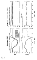
- ESP systems of a like design allow a great sideslip angle (angle ⁇ between longitudinal vehicle axle and speed vector V) in defined travel situations with an insignificant control deviation (difference between nominal and actual yaw rate), as is shown in the left half of the depict of FIG. 8.
- the sideslip angle may be limited if the driver increases the control deviation by steering corrections and, consequently, causes a major control intervention of the yaw rate control.
- An object of the present invention is to improve the quality of the control and reduce the demands placed on the driver.
- this is achieved by passing from the one-quantity control to a multiple-quantities control. It is utilized in this respect that the lateral-dynamics state of the vehicle in a first approximation is characterized by the two quantities ‘yaw rate ⁇ dot over ( ⁇ ) ⁇ ’ and ‘sideslip angle ⁇ ’. These quantities are illustrated in FIG. 1. From a present point of view, it is unfavorable under economical aspects to directly measure the sideslip angle for future ESP systems. Instead, attempts are made to estimate the sideslip angle based on the signals of the available sensor equipment.
- the method is characterized by the following step:
- the predicted vehicle state variables ⁇ circumflex over (x) ⁇ for the next sampling moment t k+1 are achieved by integration according to the non-linear equation x ⁇ ⁇ ( t k + 1
- t k ) x ⁇ ⁇ ( t k
- t k ⁇ 1 ) h m ( ⁇ circumflex over (x) ⁇ (t k
- t k ⁇ 1 ) estimated signal at the moment t k , with information of the last moment t k ⁇ 1 being used.
- t k ) ⁇ circumflex over (x) ⁇ (t k
- the method resides in the step: establishing the estimated controlled quantities y r at the moment t k by using information about the current moment from the driving dynamics quantities ⁇ circumflex over (x) ⁇ (t k
- t k ) h r ( ⁇ circumflex over (x) ⁇ (t k
- t k ),u m (t k )), where u m (t k ) vector of the sensed discrete input quantities.
- the method is favorable due to the step: determining the estimated control quantities y r at the moment t k by using information of the last moment from the vehicle state variables ⁇ circumflex over (x) ⁇ (t k
- t k ⁇ 1 ) h r ( ⁇ circumflex over (x) ⁇ (t k
- t k ⁇ 1 ),u m (t k )), where u m (t k ) vector of the sensed discrete input quantities.
- the method is advantageously used in a driving dynamics control, especially ESP control or suspension control.
- a generic driving dynamics control is characterized by a
- deactivation logic ( 405 ) for deactivating the sideslip angle control in dependence on the input quantities ⁇ circumflex over ( ⁇ ) ⁇ v , ⁇ circumflex over ( ⁇ ) ⁇ h and/or quantities representative of travel situations of the motor vehicle, such as rearward driving, driving around a steep turn, and the like
- An object of the present invention is to estimate controlled quantities of adequate precision and suitable for driving dynamics control (which correspond to the vehicle state quantities or permit being directly derived therefrom) such as yaw rate, sideslip angle, roll angle, pitch angle with an estimation method based on a non-linear vehicle model and by using tire or wheel forces.
- the tire or wheel forces may favorably be measured during driving by using the tire with a sidewall torsion sensor.
- the ‘sidewall torsion (SWT) sensor’ is based on the idea of measuring the deformation of the tire by means of sensors on the vehicle body and to conclude from this deformation, in view of the elastic properties, to the forces that act.
- the conventional ESP system was coupled to the SWT tire sensor equipment and extended by a sideslip angle control (that is not dependent on the SWT tire sensor equipment, however) in a favorable embodiment.
- the longitudinal tire or wheel forces F x and lateral tire or wheel forces F y are known, which assist a model in the estimation of the sideslip angle and achieve a quality of the sideslip angle estimation that is sufficient for a control.
- This combined yaw rate control and sideslip angle control renders it possible to provide a more sensitive stability control that is still more capable with respect to the average driver. Those sideslip angles which are considered unpleasant or can no longer be tackled by the driver starting from a defined magnitude are prevented. The steering effort in situations being critical in terms of driving dynamics is considerably reduced.
- the sideslip angle in the ESP with sideslip angle control is limited to a quantity that can be mastered by an average driver.
- the measure and estimated sideslip angle correspond to each other with sufficient accuracy on account of the estimation based on tire force or wheel force. No additional steering activities are required from the driver (cf. FIG. 8).
- the model-based linking of signals of low-cost sensors permits estimating signals (e.g. sideslip angle) which are required for a driving dynamics control and up to now were impossible to measure at low cost. Based on these estimated controlled quantities, among others, the following new driving dynamics control structures are possible:
- New driving stabilization control structures connected with an improvement of control quality due to a sideslip angle control or multiple-quantities control (combined yaw rate/sideslip angle control with a specification of reference values for sideslip angle and yaw rate).
- FIG. 1 shows exemplarily circumferential wheel forces (longitudinal forces) F x and lateral forces F y in the wheel-related systems of coordinates in relation to the wheel hub centers.
- An SWT sensor is used to determine the forces, using a magnet principle for measuring the deformation of the tire or the wheel, respectively.
- a special hard magnetic rubber compound was developed for the SWT encoder and is embedded in the tire sidewall. The rubber compound is magnetized after the vulcanization of the tire. North and south poles alternate in the pole patterns that result (DE 196 20 581).
- Two active magnetic field sensors mounted on the chassis measure the way the magnetic field changes as the tire rotates. Signals that permit being evaluated up to very low speeds are obtained by the selection of active sensors.
- the signal amplitude is irrespective of the rotational speed of the tire, which is in contrast to inductive sensors.
- the longitudinal deformation may be calculated from the phase difference between the two sensor signals.
- the amplitude changes reversely to the distance between sensors and sidewall, thus permitting the lateral deformation of the corners (tires, wheel hub, suspension) to be determined by said amplitude. Longitudinal and lateral forces are calculated from the two deformation components.
- the raw signals gathered by the SWT sensor are filtered and amplified before they are relayed to a central evaluating electronic unit.
- the evaluating unit the phase difference and the signal amplitude is determined, and the force components are calculated therefrom by means of a digital signal processor.
- the information about force is then relayed to the control system where other quantities are estimated by means of a vehicle model, said quantities being important to describe the driving situation (see below).
- tire or wheel forces may also be determined directly or indirectly, with the help of further or other appropriate sensor equipment, by way of a suitable mathematic conversion such as force measuring wheel rims, tire-sidewall torsion sensors, surface sensors, determination of clamping force/clamping pressure from actuating signals of the brake actuator by way of a mathematic model or clamping force/pressure measurement of the brake actuator (circumferential forces), spring travel sensors or pressure sensors in air springs or wheel load model (cf. equation F4.9) from information about lateral and longitudinal acceleration (vertical forces)
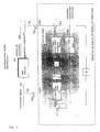
- FIG. 2 illustrates the general block wiring diagram of the process for the estimation of the states of the vehicle and the controlled quantities derived from said estimation.
- Measurable inputs u (e.g. steering angle), which may be determined by customary sensors, and/or non-measurable inputs z that can be measured with great effort only (e.g. side wind) act on the real vehicle.
- the outputs of the vehicle describing the reaction of the vehicle to the inputs are subdivided into the measurable outputs y (e.g. lateral tire forces) and the controlled quantities y r (e.g. yaw rate, sideslip angle, king pin inclination, roll angle) required for the control of driving dynamics.
- measurement variables for improving the estimation may be integrated into the process in addition to the tire or wheel forces.
- These measurement variables may be variables such as lateral/longitudinal acceleration, rotational wheel speeds, yaw rate, roll rate, and/or pitch rate.
- the measurable outputs y and the controlled quantities y r may correspond to each other in individual quantities, depending on the sensor's equipment, e.g. when using a yaw rate sensor and a combined yaw rate/sideslip angle control.
- the yaw rate is both a measurable output and a controlled quantity in this case.
- the method for the estimation of the driving dynamics quantities permits estimating controlled quantities at a rate of precision sufficient for driving dynamics control. It will be appreciated for the estimation process to be as insensitive as possible to the non-measurable inputs and modeling errors.
- a non-linear model of the vehicle (FIGS. 2 and 2 a , shaded in grey) is the basis of the estimation method.
- the estimated driving state variables or driving dynamics quantities ⁇ circumflex over (x) ⁇ may be determined by means of the continuous, non-linear system equations f( ⁇ circumflex over (x) ⁇ (t),u(t)) of the vehicle (differential equation system of first order).
- t k ⁇ 1 ) are calculated by way of the discrete, non-linear initial equations h r ( ⁇ circumflex over (x) ⁇ (t k
- a non-linear tire model for determining the tire forces from the vehicle states is also contained in the equations for the vehicle model.
- An error signal e(t k ) is generated by means of a comparison between the measured output quantities y m (t k ) (e.g. lateral forces of the tires) and the estimated measured variables ⁇ m (t k
- the state variables ⁇ circumflex over (x) ⁇ of the non-linear vehicle model are corrected with the feedback of this error signal e(t k ) by way of a gain matrix K.
- the model is adapted and the estimation improved by this feedback of the measured variables.
- the measured variables available (sensor equipment) and the quality of the sensor signals hence influence the quality of the estimation. If, for example, in addition to the tire forces other measured variables are included in the estimation, this will improve the estimation of the controlled quantities due to the linking operation by way of the vehicle model. This renders it possible for example to estimate a yaw rate with a higher rate of precision, although the used yaw rate senor may be reduced in its quality compared to the current system.
- other high-quality measured variables e.g. current yaw rate sensor and lateral acceleration sensor
- the estimation can be stabilized by the feedback of the error signal even in a vehicle model that is unstable on account of the operating point.
- the estimation is prevented from drifting due to a sensor offset, as is possible e.g. in a free integration.
- the method renders it possible to estimate forces and torques (non-measurable inputs) that act on the vehicle. Transformed to the center of gravity, the disturbing force F d and the disturbing torque T d are plotted in FIG. 1 exemplarily for the driving dynamics. The estimation of a disturbance variable is dealt with more closely in this embodiment.
- the measurable inputs u and the measurable outputs y of the real vehicle are gathered by the measurement value detection of the digital control processor (e.g. the driving dynamics controller) at discrete moments t k with the sampling time T A .
- the input disturbances w(t k ) and output disturbances v(t k ) such as sensor noises or quantization effects of the A/D converter are superposed.
- the sensed, discrete measured variables 1 u m (t k ) and y m (t k ) are used for the method to estimate the controlled quantities.
- t k ⁇ 1 ) are calculated from the predicted states ⁇ circumflex over (x) ⁇ (t k
- the error signal e(t k ) between measured and estimated measured variables (F3.2) along with the gain matrix K leads to a correction of the predicted states (F3.3).
- t k ⁇ 1 ) are determined by means of the discrete, non-linear initial equation h r (.) (F3.4.or F3.4.2).
- K time-responsive, operating-point-responsive gain matrix
- the discretized form of the integration pursuant equation F3.5 may e.g. be implemented by a simple gamma function (‘Euler-Ansatz’).
- the feedback gain matrix K can be determined at any moment t k according to equation F3.7 in dependence on two criteria
- ⁇ estimated operating point of the non-linear vehicle model.
- the information content of a sensor signal is e.g. determined by the quality of the sensor (precision, noise, drift), the position of installation (superposed vibrations, turns of the coordinates) and the modeling error of the vehicle model, meaning: how well does the measured quantity ‘fit’ to the mathematic approach.
- the elements of the return gain matrix K are selected in such a way that each measured output, depending on its information content, is optimally used for the correction of the estimated vehicle states.
- a sensor signal of low quality e.g. has also little influence on the estimation of the controlled quantities. If the information content does not change with time, consequently, no time derivative of K will result. However, it is also possible to adapt a detected change of a sensor signal (e.g. failure, increased noise) accordingly in the feedback gain matrix.
- the dynamic behavior of the vehicle is significantly responsive to the vehicle condition.
- the feedback gain matrix K to the operating point, that means estimated states, measured/estimated outputs, and/or controlled quantities. This may occur with respect to each sampling step or in defined operating ranges (e.g. saturation /no saturation of the tire characteristic curve, high/low speed).
- FIG. 3 illustrates the general structure of the disclosed lateral dynamics control (yaw torque control) based on the estimated controlled quantities sideslip angle ⁇ circumflex over ( ⁇ ) ⁇ and yaw rate ⁇ circumflex over ( ⁇ dot over ( ⁇ ) ⁇ ) ⁇ .
- yaw torque control yaw torque control
- a signal of a yaw rate sensor of lower quality is included as an input in the estimation of controlled quantities.
- the estimated yaw rate has a higher quality than the measured yaw rate what is due to the fact that information of other input quantities and measured variables is utilized.
- the calculated substitute signal ⁇ dot over ( ⁇ ) ⁇ linear in conjunction with the linearity flag may be used to improve the estimation of the controlled quantities.
- This substitute signal known from the current ESP system for monitoring the yaw rate sensor is produced from the difference wheel speeds of an axle, or the stationary steering model, or the lateral acceleration. However, this substitute signal applies only in the linear working range of vehicle dynamics.
- the corresponding elements of the feedback matrix K may then be set to zero, for example.
- Control with the Measured Yaw Rate ⁇ dot over ( ⁇ ) ⁇ This configuration is suitable when a sensor of up-to-date quality comprised in the standard ESP system is employed.
- the measured yaw rate is included in the estimation of controlled quantities for improving the estimated sideslip angle, and the measured quantity instead of the estimated quantity may be used to produce the actuating variable D ⁇ dot over ( ⁇ ) ⁇ .
- the controller structure known from series is achieved. It is conceivable in this configuration to manage without the lateral tire or wheel forces F yi as measured variables, with a tolerable reduction of the quality of the estimated sideslip angle. This is especially suitable for brake-by-wire systems that permit detecting the longitudinal tire forces upon actuation of the brake actuator without any additional sensor equipment.
- the combined yaw rate/sideslip angle control may be implemented with all yaw rate configurations (table A, FIG. 3) and is preferred over the pure yaw rate control.
- the yaw torque controller comprises a non-linear dynamic controller G b which as an input receives the actuating variable Db between the estimated sideslip angle ⁇ circumflex over ( ⁇ ) ⁇ and the reference sideslip angle b ref , and a non-linear dynamic controller G ⁇ dot over ( ⁇ ) ⁇ , which as an input receives the actuating variable ⁇ dot over ( ⁇ ) ⁇ between measured/estimated yaw rate and reference yaw rate ⁇ dot over ( ⁇ ) ⁇ re ⁇ .
- the estimated king pin inclinations ⁇ circumflex over ( ⁇ ) ⁇ V , ⁇ circumflex over ( ⁇ ) ⁇ H of the front and rear axle may be used as a controlled quantity.
- the two output quantities of the controllers are added to an additional yaw torque T req being subsequently (not shown in FIG. 3) distributed to the wheels as a brake force requirement.
- the reference value ⁇ dot over ( ⁇ ) ⁇ re ⁇ for the yaw rate is produced from a dynamic one-track model as in the standard ESP.
- the reference value ⁇ re ⁇ for the sideslip angle may also be produced by means of a dynamic model. In the normal operating range of the vehicle, however, the sideslip angle is small ( ⁇ 2°) so that an activation threshold is sufficient as ⁇ re ⁇ .
- a specification from a dynamic model is not necessary.
- the parameters or activation thresholds of the non-linear dynamic controller are adapted to the respective driving condition among others as a function of the speed V x , the yaw rate ⁇ dot over ( ⁇ ) ⁇ or ⁇ circumflex over ( ⁇ dot over ( ⁇ ) ⁇ ) ⁇ , respectively, the estimated sideslip angles and king pin inclinations ⁇ circumflex over ( ⁇ ) ⁇ , ⁇ circumflex over ( ⁇ ) ⁇ V , ⁇ circumflex over ( ⁇ ) ⁇ H and the coefficient of friction.
- the generation of the sideslip angle reference value and the adaptation of the sideslip angle controller G b is described.
- a preferred embodiment due to a performance which is significantly improved in comparison to the known ESP system is directed to the combined yaw rate/sideslip angle control by using a yaw rate sensor of identical quality or a quality reduced compared to up-to-date sensors (right column, table A, FIG. 3).
- the following example describes a favorable embodiment of the present invention comprising the estimation of the lateral dynamics conditions ‘yaw rate’ and ‘sideslip angle’ and the combined yaw rate/sideslip angle control based thereon.
- a yaw rate sensor signal is available for the estimation and control.
- the basis for the estimation of yaw rate and sideslip angle is a plane two-track model for the lateral dynamics movement by neglecting roll and pitch dynamics.
- the effect of rolling and pitching is taken into consideration in the tire model by way of the influence of the vertical wheel force.
- ⁇ circumflex over (x) ⁇ [ ⁇ circumflex over (V) ⁇ y , ⁇ circumflex over ( ⁇ dot over ( ⁇ ) ⁇ ) ⁇ , ⁇ circumflex over (F) ⁇ d ] T estimated states of the vehicle
- the measurable inputs u are the longitudinal vehicle speed V x which is a quantity estimated in the standard ESP based on the wheel speeds, the steering angle ⁇ , the four longitudinal tire or wheel forces F x , the four vertical forces ⁇ circumflex over (F) ⁇ z , calculated pursuant equation F4.9 and the four coefficients of friction ⁇ circumflex over ( ⁇ ) ⁇ i for the tire/road contact.
- the coefficients of friction may e.g. be either adopted from the estimated frictional value of the standard ESP, or may be determined by a special estimation algorithm, e.g. from the tire forces or quantities derived therefrom, in pairs or per wheels.
- the outputs y m or ⁇ , respectively, are the four lateral tire or wheel forces F y , the lateral acceleration a y preferably in the center of gravity or in the sensor position, and the yaw rate ⁇ dot over ( ⁇ ) ⁇ .
- the estimated controlled quantities ⁇ r are the sideslip angle ⁇ circumflex over ( ⁇ ) ⁇ , the king pin inclination for front and rear axles ⁇ circumflex over ( ⁇ ) ⁇ v , ⁇ circumflex over ( ⁇ ) ⁇ h , and the yaw rate ⁇ circumflex over ( ⁇ dot over ( ⁇ ) ⁇ ) ⁇ .
- the estimated states ⁇ circumflex over (x) ⁇ are the lateral vehicle speed ⁇ circumflex over (V) ⁇ y , the yaw rate ⁇ circumflex over ( ⁇ dot over ( ⁇ ) ⁇ ) ⁇ , and the disturbing force ⁇ circumflex over (F) ⁇ d (cf. FIG. 1), which shall be estimated as a non-measurable input (e.g. wind force, impact).
- the disturbance variable it is interpreted as a state x 3 and included in the state vector x. This procedure is equivalently possible for further disturbance variables such as the disturbing torque T d and/or unknown or changing parameters (mass of the vehicle, coefficient of friction tire/road).
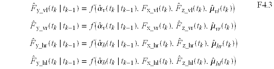
- the tire model pursuant equation F4.3 depicts the non-linear characteristics of the characteristic curve of the lateral tire force, as it is illustrated in FIG. 5 principally as a function of the essential influencing variables.
- This characteristic curve may be plotted in tables, or preferably analytically in the way of e.g. an approximated polynomial.
- t k ) h r ( ⁇ circumflex over (x) ⁇ (t k
- t k ),u m (t k )) may be determined with the updated states pursuant equation F3.4 by means of the non-linear initial equation.
- y ⁇ r1 ⁇ ⁇ ⁇ ( t k
- t k ) V ⁇ y ⁇ ( t k
- t k ) V x ⁇ ( t k ) y ⁇ r2 ⁇ ⁇ v ⁇ ( t k
- t k ) y ⁇ r3 ⁇ ⁇ h ⁇ ( t k
- t k ) y ⁇ r4 ⁇ ⁇ . ⁇ ( t k
- t k - 1 ) - ⁇ ⁇ ( t k ) + V ⁇ y ⁇ ( t k
- t k - 1 ) V ⁇ y ⁇ ( t k
- the estimated controlled quantity ⁇ circumflex over ( ⁇ dot over ( ⁇ ) ⁇ ) ⁇ is not used in the subsequent embodiment for the controller because a yaw rate sensor of up-to-date quality is made the basis.
- FIG. 6 illustrates the characteristic curve according to equation F4.8.
- the hatched band marks the zone of small sideslip angles of the vehicle that can still be easily mastered by the driver. No control intervention due to excessive sideslip angles is necessary within this zone
- the control entry threshold is reduced to a limit value b limit,ref because large sideslip angles are more difficult for the driver to master at higher speeds.
- Typical values for the characteristic curve of the control entry threshold b ref are:
- a stationary model pursuant equation (F4.9) is used in block 403 for estimating the vertical forces.
- the vertical forces F z are estimated with the longitudinal and lateral accelerations a x and a y applied to the center of gravity.
- the longitudinal acceleration may be a quantity measured by a sensor as well as a quantity estimated from the wheel speeds, e.g. in the standard ESP.
- F ⁇ z_vl m l ⁇ ( l h ⁇ g - h ⁇ ⁇ a ⁇ x ) ⁇ ( 1 2 - h b v ⁇ g ⁇ a y )
- F ⁇ z_vr m l ⁇ ( l h ⁇ g - h ⁇ ⁇ a ⁇ x ) ⁇ ( 1 2 + h b v ⁇ g ⁇ a y )
- F ⁇ z_hl m l ⁇ ( l v ⁇ g + h _ ⁇ ⁇ a ⁇ x ) ⁇ ( 1 2 - h b h ⁇ g ⁇ a y )
- F ⁇ z_hr m l ⁇ ( l v ⁇ g - h ⁇ ⁇ a ⁇ x ⁇ ( 1 2 + h b h ⁇ g ⁇
- an additional yaw torque stabilizing the vehicle is calculated according to equation (F4.11) from the sideslip angle difference
- T req_beta ⁇ f ⁇ ( ⁇ ⁇ , ⁇ ⁇ ⁇ ⁇ , V x , ⁇ . , ⁇ ⁇ ⁇ ⁇ . , ⁇ ) ⁇ for ⁇ ⁇ > ⁇ ref , ⁇ . ⁇ 0 , V x > V min ⁇ for ⁇ ⁇ ⁇ - ⁇ ref , ⁇ . > 0 , V x > V min 0 otherwise F4 . ⁇ 11
- An additional torque T req — beta is calculated when the estimated sideslip angle ⁇ circumflex over ( ⁇ ) ⁇ lies outside the band limited by b ref , as shown in FIG. 6.
- the direction of the yaw rate is another condition.
- ⁇ circumflex over ( ⁇ ) ⁇ > ⁇ re ⁇ and ⁇ dot over ( ⁇ ) ⁇ >0 an additional torque becomes unnecessary. No control is required below a speed V min .
- the additional torque is preferably calculated proportionally in relation to the deviation Db.
- FIG. 7 a typical variation of the required additional torque T req — beta in dependence on the deviation Db is shown.
- the zero torque T 0,req — beta is necessary in order to achieve a significant additional yaw torque for driving stabilization when the control commences.
- the sideslip angle control is deactivated during rearward driving or when driving around a steep turn and if the difference between the king pin inclinations at the front and rear axles is large, i.e.,
- the nominal values of the wheel brake pressure are determined from the required additional torque in a way similar to the standard ESP.
- the difference compared to the standard ESP involves that with the sideslip angle control active, pressure is also required on the rear wheels in addition to the pressure requirement on the front wheels. In this respect, a distinction is made as to whether the sideslip angle control is active alone, or whether the standard ESP is active in addition.
Abstract
The present invention relates to a method for the online determination of values of driving dynamics for a motor vehicle.
To improve the quality of the control of a motor vehicle and to reduce the demands placed on the driver, the invention discloses a driving dynamics control including the following steps:
Determining estimated output quantities ŷm in dependence on determined and/or estimated input quantities u and predetermined or predicted vehicle state variables {circumflex over (x)} and optionally further quantities,
comparing the estimated output quantities ŷm with measured output quantities ym, and
determining the estimated driving dynamics quantities {circumflex over (x)}(tk/tk) in dependence on the measurement result and, as the case may be, further criteria.
Description
- The present invention relates to a method for the online determination of values of driving dynamics for a motor vehicle, a driving dynamics control, and use of the method and the driving dynamics control.
- An ESP system with yaw rate control represents the state of the art, the control being based on a precise yaw rate sensor that is expensive compared to the overall system. Prior art ABS, TCS, and driving dynamics control systems (such as ESP=Electronic Stability Program) assess the signals from wheel speed sensors (ABS, TCS) and from sensors related to additional specifications of the driver and driving dynamics sensors (ESP) in order to detect and reliably master unstable vehicle movements. The specifications, as defined by the driver, are detected by means of a steering angle sensor, pressure sensors in the master brake cylinder, and the engine management. Typical driving dynamics sensors are a lateral acceleration sensor and, in a four-wheel drive, possibly a longitudinal acceleration sensor. The sensor that is most important for ESP is the yaw rate sensor measuring the rotational speed of the vehicle about the vertical axis.
- Driving dynamics control is implemented as a control for the yaw rate {dot over (ψ)}. The nominal value of the yaw rate is generated online by means of a one-track vehicle model. ESP systems of a like design allow a great sideslip angle (angle β between longitudinal vehicle axle and speed vector V) in defined travel situations with an insignificant control deviation (difference between nominal and actual yaw rate), as is shown in the left half of the depict of FIG. 8. The sideslip angle may be limited if the driver increases the control deviation by steering corrections and, consequently, causes a major control intervention of the yaw rate control.
- An object of the present invention is to improve the quality of the control and reduce the demands placed on the driver.
- Advantageously, this is achieved by passing from the one-quantity control to a multiple-quantities control. It is utilized in this respect that the lateral-dynamics state of the vehicle in a first approximation is characterized by the two quantities ‘yaw rate {dot over (ψ)}’ and ‘sideslip angle β’. These quantities are illustrated in FIG. 1. From a present point of view, it is unfavorable under economical aspects to directly measure the sideslip angle for future ESP systems. Instead, attempts are made to estimate the sideslip angle based on the signals of the available sensor equipment.
- According to the present invention, this object is achieved in a generic method by the following steps:
- Determining estimated output quantities ŷ m in dependence on determined and/or estimated input quantities u and predetermined or predicted vehicle state variables {circumflex over (x)} and optionally further quantities, comparing the estimated output quantities ŷm with measured output quantities ym, and determining the estimated quantities of driving dynamics {circumflex over (x)}(tk/tk) in dependence on the comparison result and, as the case may be, further criteria.
- In a favorable aspect of this invention, the method is characterized by the following step:
- model-based determination of the predicted vehicle state variables {circumflex over (x)} in dependence on determined and/or estimated input quantities u and the driving dynamics quantities {circumflex over (x)}(t k/tk).
- In this arrangement, the following input quantities u(t)={circumflex over (V)} x, δ, Fx; {circumflex over (F)}z or Fz, {circumflex over (μ)}i or μi are preferably taken into account in the estimation of the predicted vehicle state variables {circumflex over (x)} and in the determination of the driving dynamics quantities {circumflex over (x)}(tk/tk), where {circumflex over (V)}x=estimated longitudinal vehicle speed, δ=the measured steering angle, Fx=the determined longitudinal tire or wheel forces, {circumflex over (F)}z=the estimated vertical forces, or {circumflex over (F)}z=the determined vertical forces, {circumflex over (μ)}i=the estimated coefficients of friction for the tire/road contact, or μi=the determined coefficients of friction for the tire/road contact. As driving dynamics quantities and the predicted vehicle state variables {circumflex over (x)}=[{circumflex over (V)}y, {circumflex over ({dot over (ψ)})}, {circumflex over (F)}d]T the lateral vehicle speed {circumflex over (V)}y, the yaw rate {circumflex over ({dot over (ψ)})} and the disturbing forces {circumflex over (F)}d, which are estimated as non-measurable input quantities, are preferably determined.
- As other quantities of driving dynamics and the predicted vehicle state variables {circumflex over (x)}=[{circumflex over (T)} d, μi]T the disturbing torques Md and the coefficients of friction μi are determined as non-measurable input quantities.
- Advantageously, the predicted vehicle state variables {circumflex over (x)} for the next sampling moment t k+1 are achieved by integration according to the non-linear equation

- with the start condition {circumflex over (x)}(t k/tk), where
- {circumflex over (x)} estimated state vector,
- f(.) continuous, non-linear system equations
- x(t k) signal at the discrete moment tk. (current moment)
- {circumflex over (x)}(t k|tk−1) estimated signal at the moment tk, with only information of the last moment tk−1 used
- {circumflex over (x)}(t k|tk) estimated signal at the moment tk, with only information of the current moment tk used
- {circumflex over (x)}(t k+1|tk) predicted signal for the next moment tk+1, with only information of the current moment tk used
- t k discrete moment.
- It is appropriate that as an output quantity ŷ m=[{circumflex over (α)}y] the lateral acceleration ay is estimated.
- It is also appropriate that as another output quantity ŷ m=[{dot over (ψ)}] the yaw rate {dot over (ψ)} is estimated.
- In addition, it is appropriate that as still other output quantities ŷ m=[{circumflex over (F)}y]T the lateral tire and wheel forces Fy. are estimated.
- It is favorable that the output quantities ŷ m for the sampling moment tk are estimated according to the discrete, non-linear equation hm
- Ŷm(tk|tk−1)=hm({circumflex over (x)}(tk|tk−1),um(tk))
- from the vehicle state variables {circumflex over (x)}(t k|tk−1) and the input quantities um(tk), where
- ŷ m estimated output vector of the measurable outputs
- {circumflex over (x)} estimated state vector,
- u m input vector of the measurable inputs
- h m(.) discrete, non-linear measurement equations
- {circumflex over (x)}(t k|tk−1) estimated signal at the moment tk, with only information of the last moment tk−1 being used
- ŷ(t k|tk−1) estimated signal at the moment tk, with only information of the last moment tk−1 used
- t k discrete moment.
- It is especially suitable that at least one of the estimated output quantities ŷ m=[{circumflex over (F)}y, {circumflex over (α)}y, {circumflex over ({dot over (ψ)})}]T is compared to at least one of the determined (acquired directly or indirectly by means of sensors) output quantities ym(tk)=[Fy,αy, {dot over (ψ)}]T and the comparison results e(tk) are sent to a summation point, preferably by way of a gain matrix K, for the correction of the vehicle state variable {circumflex over (x)}(tk|tk−1), where {circumflex over (x)}(tk|tk−1)=estimated signal at the moment tk, with information of the last moment tk−1 being used.
- It is advantageous that the gain matrix K at every moment t k is defined pursuant the relation K(tk)=ƒ(Â, G) where G=information content of the determined (measured) signals and Â=estimated operating point of the non-linear vehicle model.
- It is favorable that the correction of the driving dynamics quantities is carried out according to the relation
- {circumflex over (x)}(tk|tk)={circumflex over (x)}(tk|tk−1)+K(tk)e(tk).
- In a particularly favorable fashion, the method resides in the step: establishing the estimated controlled quantities y r at the moment tk by using information about the current moment from the driving dynamics quantities {circumflex over (x)}(tk|tk) and the input quantities um(tk) according to the relation ŷr(tk|tk)=hr({circumflex over (x)}(tk|tk),um(tk)), where um(tk)=vector of the sensed discrete input quantities.
- Further, the method is favorable due to the step: determining the estimated control quantities y r at the moment tk by using information of the last moment from the vehicle state variables {circumflex over (x)}(tk|tk−1) and the input quantities um(tk) pursuant the relation ŷr(tk|tk−1)=hr({circumflex over (x)}(tk|tk−1),um(tk)), where um(tk)=vector of the sensed discrete input quantities.
- A particularly favorable multiple-quantities control is achieved by means of the following steps:
- determining an estimated sideslip angle {circumflex over (β)} as a controlled quantity ŷ r(tk|tk−1) or ŷr(tk|tk), respectively,
- comparing the estimated sideslip angle {circumflex over (β)} with a sideslip angle reference quantity β reƒ,
- producing an additional yaw torque T req from the estimated difference between the sideslip reference quantity βreƒ and the sideslip angle {circumflex over (β)} and a difference between a yaw rate reference quantity {dot over (ψ)}reƒ and a yaw rate {dot over (ψ)} or {circumflex over ({dot over (ψ)})} or {dot over (ψ)}linear and actuation of at least one wheel brake of the motor vehicle in dependence on the additional yaw torque Treq.
- The method is advantageously used in a driving dynamics control, especially ESP control or suspension control.
- According to the present invention, a generic driving dynamics control is characterized by a
- first determining unit ( 402) for estimating the controlled quantities {dot over (β)} and/or {circumflex over (α)}y, {circumflex over (α)}h from the input quantities Vx, δ, Fx, {dot over (ψ)}, {circumflex over (μ)}, αy, {circumflex over (F)}z and/or, if necessary, other quantities Fz, {dot over (ψ)}linear,
- deactivation logic ( 405) for deactivating the sideslip angle control in dependence on the input quantities {circumflex over (α)}v, {circumflex over (α)}h and/or quantities representative of travel situations of the motor vehicle, such as rearward driving, driving around a steep turn, and the like
- second determining unit ( 404) for the adaptive sideslip angle torque calculation from the input quantities {circumflex over (β)}, βreƒ, Vreƒ or Vx, {circumflex over (μ)}i, respectively,
- third determining unit ( 406) for the arbitration of an additional yaw torque Treq. from the yaw torque Treg
— ESP and Treg— beta. - Favorable improvements of the present invention are described in the subclaims.
- An object of the present invention is to estimate controlled quantities of adequate precision and suitable for driving dynamics control (which correspond to the vehicle state quantities or permit being directly derived therefrom) such as yaw rate, sideslip angle, roll angle, pitch angle with an estimation method based on a non-linear vehicle model and by using tire or wheel forces. The tire or wheel forces may favorably be measured during driving by using the tire with a sidewall torsion sensor. The ‘sidewall torsion (SWT) sensor’ is based on the idea of measuring the deformation of the tire by means of sensors on the vehicle body and to conclude from this deformation, in view of the elastic properties, to the forces that act.
- Depending on the demanded controlled quantities (control task) and the necessary quality of the estimation, other sensor signals related to the longitudinal, lateral and roll movements of the vehicle (e.g. lateral acceleration, wheel speeds, yaw rate and/or roll rate) may be taken into consideration in the estimation.
- New driving dynamics control systems are drafted with these estimated controlled quantities.
- For the new tire-force or wheel-force assisted driving dynamics control, the conventional ESP system was coupled to the SWT tire sensor equipment and extended by a sideslip angle control (that is not dependent on the SWT tire sensor equipment, however) in a favorable embodiment. As this occurs, the longitudinal tire or wheel forces F x and lateral tire or wheel forces Fy are known, which assist a model in the estimation of the sideslip angle and achieve a quality of the sideslip angle estimation that is sufficient for a control.
- This combined yaw rate control and sideslip angle control renders it possible to provide a more sensitive stability control that is still more capable with respect to the average driver. Those sideslip angles which are considered unpleasant or can no longer be tackled by the driver starting from a defined magnitude are prevented. The steering effort in situations being critical in terms of driving dynamics is considerably reduced.
- This becomes clear when comparing a driving maneuver with a standard ESP with a maneuver with ESP with sideslip angle control. In a circling movement of a vehicle in the critical range on snow, a sideslip angle develops in the standard ESP as the driving force reduces, said sideslip angle allowing to be compensated only by an abrupt steering reaction (FIG. 8, left hand side). The information about the yaw rate alone is not sufficient for stabilizing.
- In contrast thereto, the sideslip angle in the ESP with sideslip angle control is limited to a quantity that can be mastered by an average driver. The measure and estimated sideslip angle correspond to each other with sufficient accuracy on account of the estimation based on tire force or wheel force. No additional steering activities are required from the driver (cf. FIG. 8).
- 2. Advantages of the Present Invention
- The model-based linking of signals of low-cost sensors permits estimating signals (e.g. sideslip angle) which are required for a driving dynamics control and up to now were impossible to measure at low cost. Based on these estimated controlled quantities, among others, the following new driving dynamics control structures are possible:
- Replacement of the yaw rate sensor (cost reduction). The signal is determined by an estimated quantity. The known ESP system is maintained in its structure.
- New driving stabilization control structures connected with an improvement of control quality due to a sideslip angle control or multiple-quantities control (combined yaw rate/sideslip angle control with a specification of reference values for sideslip angle and yaw rate).
- New active steering systems on the basis of the sideslip angle determination.
- 3. Description of the Method
- In the following, the method for the estimation of the states and the controlled quantities of the vehicle derived therefrom, as well as the structure of the driving dynamics control will be explained which is based on the estimated controlled quantities.
- 3.1. Estimation of the Controlled Quantities
- The forces developing due to the tire/road contact and acting on the vehicle are used for the method. These forces may be circumferential wheel forces, lateral forces, and/or vertical wheel forces. FIG. 1 shows exemplarily circumferential wheel forces (longitudinal forces) F x and lateral forces Fy in the wheel-related systems of coordinates in relation to the wheel hub centers. An SWT sensor is used to determine the forces, using a magnet principle for measuring the deformation of the tire or the wheel, respectively. A special hard magnetic rubber compound was developed for the SWT encoder and is embedded in the tire sidewall. The rubber compound is magnetized after the vulcanization of the tire. North and south poles alternate in the pole patterns that result (DE 196 20 581). Two active magnetic field sensors mounted on the chassis measure the way the magnetic field changes as the tire rotates. Signals that permit being evaluated up to very low speeds are obtained by the selection of active sensors. The signal amplitude is irrespective of the rotational speed of the tire, which is in contrast to inductive sensors. The longitudinal deformation may be calculated from the phase difference between the two sensor signals. The amplitude changes reversely to the distance between sensors and sidewall, thus permitting the lateral deformation of the corners (tires, wheel hub, suspension) to be determined by said amplitude. Longitudinal and lateral forces are calculated from the two deformation components. In addition, it is possible to determine the wheel speed with only one sensor, in the same manner as with an ABS sensor. The raw signals gathered by the SWT sensor are filtered and amplified before they are relayed to a central evaluating electronic unit. In the evaluating unit the phase difference and the signal amplitude is determined, and the force components are calculated therefrom by means of a digital signal processor. The information about force is then relayed to the control system where other quantities are estimated by means of a vehicle model, said quantities being important to describe the driving situation (see below).
- These tire or wheel forces may also be determined directly or indirectly, with the help of further or other appropriate sensor equipment, by way of a suitable mathematic conversion such as force measuring wheel rims, tire-sidewall torsion sensors, surface sensors, determination of clamping force/clamping pressure from actuating signals of the brake actuator by way of a mathematic model or clamping force/pressure measurement of the brake actuator (circumferential forces), spring travel sensors or pressure sensors in air springs or wheel load model (cf. equation F4.9) from information about lateral and longitudinal acceleration (vertical forces)
- General Description of the Estimation Process
- FIG. 2 illustrates the general block wiring diagram of the process for the estimation of the states of the vehicle and the controlled quantities derived from said estimation.
- Measurable inputs u(e.g. steering angle), which may be determined by customary sensors, and/or non-measurable inputs z that can be measured with great effort only (e.g. side wind) act on the real vehicle. The outputs of the vehicle describing the reaction of the vehicle to the inputs are subdivided into the measurable outputs y (e.g. lateral tire forces) and the controlled quantities y r (e.g. yaw rate, sideslip angle, king pin inclination, roll angle) required for the control of driving dynamics.
- Other measurement variables for improving the estimation may be integrated into the process in addition to the tire or wheel forces. These measurement variables may be variables such as lateral/longitudinal acceleration, rotational wheel speeds, yaw rate, roll rate, and/or pitch rate. The measurable outputs y and the controlled quantities y r may correspond to each other in individual quantities, depending on the sensor's equipment, e.g. when using a yaw rate sensor and a combined yaw rate/sideslip angle control. The yaw rate is both a measurable output and a controlled quantity in this case.
- With the knowledge of the measurable inputs and outputs of the real vehicle—corresponding to the sensor' equipment—the method for the estimation of the driving dynamics quantities permits estimating controlled quantities at a rate of precision sufficient for driving dynamics control. It will be appreciated for the estimation process to be as insensitive as possible to the non-measurable inputs and modeling errors.
- This may be achieved by the method presented in the following:
- A non-linear model of the vehicle (FIGS. 2 and 2 a, shaded in grey) is the basis of the estimation method. The estimated driving state variables or driving dynamics quantities {circumflex over (x)} may be determined by means of the continuous, non-linear system equations f({circumflex over (x)}(t),u(t)) of the vehicle (differential equation system of first order). Based on these driving state variables or driving dynamics quantities, the estimated controlled quantities ŷr(tk|tk) or ŷr(tk|tk−1) are calculated by way of the discrete, non-linear initial equations hr({circumflex over (x)}(tk|tk),um(tk)) or hr({circumflex over (x)}(tk|tk−1),um(tk)). A non-linear tire model for determining the tire forces from the vehicle states is also contained in the equations for the vehicle model.
- An error signal e(t k) is generated by means of a comparison between the measured output quantities ym(tk) (e.g. lateral forces of the tires) and the estimated measured variables ŷm(tk|tk−1) being calculated from the estimated vehicle state variables {circumflex over (x)} by means of the discrete non-linear measurement equations hm({circumflex over (x)}(tk|tk−1),um(tk)). The state variables {circumflex over (x)} of the non-linear vehicle model are corrected with the feedback of this error signal e(tk) by way of a gain matrix K. The model is adapted and the estimation improved by this feedback of the measured variables.
- The measured variables available (sensor equipment) and the quality of the sensor signals hence influence the quality of the estimation. If, for example, in addition to the tire forces other measured variables are included in the estimation, this will improve the estimation of the controlled quantities due to the linking operation by way of the vehicle model. This renders it possible for example to estimate a yaw rate with a higher rate of precision, although the used yaw rate senor may be reduced in its quality compared to the current system. When using other high-quality measured variables (e.g. current yaw rate sensor and lateral acceleration sensor), it is conceivable as an alternative to employ tire or wheel force signals of reduced quality or to manage without the feedback of the lateral tire or wheel forces when reduced estimation accuracy is tolerated.
- Further, the estimation can be stabilized by the feedback of the error signal even in a vehicle model that is unstable on account of the operating point. Thus, the estimation is prevented from drifting due to a sensor offset, as is possible e.g. in a free integration. Further, the method renders it possible to estimate forces and torques (non-measurable inputs) that act on the vehicle. Transformed to the center of gravity, the disturbing force F d and the disturbing torque Td are plotted in FIG. 1 exemplarily for the driving dynamics. The estimation of a disturbance variable is dealt with more closely in this embodiment.
- Description of the Estimation Equations (cf. FIGS. 2 and 2 a)
- The measurable inputs u and the measurable outputs y of the real vehicle are gathered by the measurement value detection of the digital control processor (e.g. the driving dynamics controller) at discrete moments t k with the sampling time TA. In addition, the input disturbances w(tk) and output disturbances v(tk) such as sensor noises or quantization effects of the A/D converter are superposed. The sensed, discrete measured variables1 um(tk) and ym(tk) are used for the method to estimate the controlled quantities.
- 1Nomenclature of the correlations with respect to time:
- x(t k) signal at the discrete moment tk. (current moment)
- {circumflex over (x)}(t k|tk−1) estimated signal at moment tk, with only information of the last moment tk−1 used
- {circumflex over (x)}(t k|tk) estimated signal at moment tk, with information of the current moment tk used
- {circumflex over (x)}(t k+1|tk) predicted signal for the next moment tk+1, with only information of the current moment tk used.
- For each sampling step the estimated measured variables ŷ m(tk|tk−1) are calculated from the predicted states {circumflex over (x)}(tk|tk−1) and the inputs um(tk) by means of the discrete non-linear measurement equation hm(.) (F3.1). The error signal e(tk) between measured and estimated measured variables (F3.2) along with the gain matrix K leads to a correction of the predicted states (F3.3). With the corrected states {circumflex over (x)}(tk|tk) or the states of the last moment {circumflex over (x)}(tk|kk−1) the estimated controlled quantities ŷr(tk|tk) or ŷr(tk|tk−1) are determined by means of the discrete, non-linear initial equation hr(.) (F3.4.or F3.4.2). The relations {circumflex over (x)}(tk+1|t k) for the next sampling moment tk+1 are predicted according to equation F3.5 by integration of the non-linear continuous system equations f(.) with the initial relation {circumflex over (x)}(tk|tk).
- ŷ m(t k |t k−1)=h m({circumflex over (x)}( t k t k−1),u m(t k)) F3.1
- e(t k)=y m(t k)−ŷ m(t k |t k−1) F3.2
- {circumflex over (x)}(t k t k)={circumflex over (x)}(t k |t k−1)+K(t k)e(t k) F3.3
- ŷ r(t k t k)=h r({circumflex over (x)}(t k |t k),u m(t k)) F3.4.1
- ŷ r(t k |t k−1)=h r({circumflex over (x)}(t k t k−1)u m(t k)) F3.4.2
- {circumflex over (x)}(t k+1 |t k)={circumflex over (x)}(t k t k)+t
k k+1t □f({circumflex over (x)}(t),u(t))dt F3.5 - where
- t k discrete moment
- u m input vector of the measurable inputs
- y m output vector of the measurable outputs
- ŷ m estimated output vector of the measurable outputs
- ŷ r estimated output vector of the controlled quantities
- {circumflex over (x)} state vector, estimated
- h m(.) discrete, non-linear measurement equations
- h r(.) discrete, non-linear initial equations
- f(.) continuous, non-linear system equations (e.g. lateral dynamics including tire model, roll dynamics)
- e residues, difference between measured and estimated outputs
- K (time-responsive, operating-point-responsive gain matrix)
- The discretized form of the integration pursuant equation F3.5 may e.g. be implemented by a simple gamma function (‘Euler-Ansatz’).
- {circumflex over (x)}(t k+1 |t k)={circumflex over (x)}(t k |t k)+T A f({circumflex over (x)}(t k |t k),u(t k)) F3.6
- Determination of the Feedback Gain Matrix K
- The feedback gain matrix K can be determined at any moment t k according to equation F3.7 in dependence on two criteria
- G: information content of the measured signals and
- Â: estimated operating point of the non-linear vehicle model.
- K(t k)=ƒ(Â,G) F3.7
- The information content of a sensor signal is e.g. determined by the quality of the sensor (precision, noise, drift), the position of installation (superposed vibrations, turns of the coordinates) and the modeling error of the vehicle model, meaning: how well does the measured quantity ‘fit’ to the mathematic approach. The elements of the return gain matrix K are selected in such a way that each measured output, depending on its information content, is optimally used for the correction of the estimated vehicle states. Thus, a sensor signal of low quality e.g. has also little influence on the estimation of the controlled quantities. If the information content does not change with time, consequently, no time derivative of K will result. However, it is also possible to adapt a detected change of a sensor signal (e.g. failure, increased noise) accordingly in the feedback gain matrix.
- The dynamic behavior of the vehicle is significantly responsive to the vehicle condition. Under control technology aspects this means that the inherent values of the differential equation describing the vehicle vary within wide limits as a function of e.g. the vehicle speed and the operating-point-responsive lateral tire stiffness values (gradient of the characteristic curve of the lateral tire force, FIG. 5). To achieve an optimal estimation, it is suitable to adapt the feedback gain matrix K to the operating point, that means estimated states, measured/estimated outputs, and/or controlled quantities. This may occur with respect to each sampling step or in defined operating ranges (e.g. saturation /no saturation of the tire characteristic curve, high/low speed).
- 3.2 Controller Structure of Driving Dynamics Control
- The controlled quantities ‘sideslip angle’ and ‘yaw rate’ are required for controlling the lateral dynamics of the vehicle. FIG. 3 illustrates the general structure of the disclosed lateral dynamics control (yaw torque control) based on the estimated controlled quantities sideslip angle {circumflex over (β)} and yaw rate {circumflex over ({dot over (ψ)})}. When a high-quality yaw rate sensor is used, it is also possible to use the measured yaw rate {dot over (ψ)} for the control instead of the estimated yaw rate.
- The estimation of the controlled quantities sideslip angle {circumflex over (β)} and yaw rate {circumflex over ({dot over (ψ)})} is carried out according to the method that is described in sections 3.1 and 4.1. Quantities used for the estimation (cf. FIG. 3) are the inputs u m: vehicle speed Vx, steering angle δ, longitudinal tire or wheel forces Fxi, and the measured variables ym: lateral acceleration ay, the lateral tire or wheel forces Fyi, and yaw rate {dot over (ψ)}. As an alternative to the yaw rate {dot over (ψ)} it is also possible to use the substitute signal {dot over (ψ)}linear in connection with the linearity flag. Other input quantities defined outside the estimation method, which are measured by appropriate sensors or calculated or estimated from other pieces of information, are the vertical forces {circumflex over (F)}zi of each wheel and the coefficients of friction {circumflex over (μ)}i for the tire/road contact.
- Based on the sensor configuration, the suitable estimation/controller structures are illustrated in FIG. 3 (table A,B):
- Control with the Estimated Yaw Rate {circumflex over ({dot over (ψ)})} To produce the actuating variable Δ{dot over (ψ)} the estimated yaw rate {circumflex over ({dot over (ψ)})} is used. The yaw rate sensor can be economized for cost reasons or reduced in its quality.
- A signal of a yaw rate sensor of lower quality (less accuracy, offset drift) is included as an input in the estimation of controlled quantities. The estimated yaw rate has a higher quality than the measured yaw rate what is due to the fact that information of other input quantities and measured variables is utilized.
- If no yaw rate sensor is employed or the sensor has failed, the calculated substitute signal {dot over (ψ)} linear in conjunction with the linearity flag may be used to improve the estimation of the controlled quantities. This substitute signal known from the current ESP system for monitoring the yaw rate sensor is produced from the difference wheel speeds of an axle, or the stationary steering model, or the lateral acceleration. However, this substitute signal applies only in the linear working range of vehicle dynamics. In dependence on the linearity flag indicative of this validity range, the feedback for the error signal between measured and estimated yaw rate e{dot over (ψ)}={dot over (ψ)}linear −{circumflex over ({dot over (ψ)})} to the estimated states {circumflex over (x)}(tk) (see FIG. 2) is obviated. The corresponding elements of the feedback matrix K may then be set to zero, for example.
- Control with the Measured Yaw Rate {dot over (ψ)} This configuration is suitable when a sensor of up-to-date quality comprised in the standard ESP system is employed. The measured yaw rate is included in the estimation of controlled quantities for improving the estimated sideslip angle, and the measured quantity instead of the estimated quantity may be used to produce the actuating variable D{dot over (ψ)}. When the estimated sideslip angle is not used for the control, the controller structure known from series is achieved. It is conceivable in this configuration to manage without the lateral tire or wheel forces F yi as measured variables, with a tolerable reduction of the quality of the estimated sideslip angle. This is especially suitable for brake-by-wire systems that permit detecting the longitudinal tire forces upon actuation of the brake actuator without any additional sensor equipment.
- The combined yaw rate/sideslip angle control (switch B) may be implemented with all yaw rate configurations (table A, FIG. 3) and is preferred over the pure yaw rate control.
- The yaw torque controller comprises a non-linear dynamic controller G b which as an input receives the actuating variable Db between the estimated sideslip angle {circumflex over (β)} and the reference sideslip angle bref, and a non-linear dynamic controller G{dot over (ψ)}, which as an input receives the actuating variable Δ{dot over (ψ)} between measured/estimated yaw rate and reference yaw rate {dot over (ψ)}reƒ. Instead of, or in connection with, the vehicle sideslip angle β, the estimated king pin inclinations {circumflex over (α)}V,{circumflex over (α)}H of the front and rear axle may be used as a controlled quantity. The two output quantities of the controllers are added to an additional yaw torque Treq being subsequently (not shown in FIG. 3) distributed to the wheels as a brake force requirement.
- The reference value {dot over (ψ)} reƒ for the yaw rate is produced from a dynamic one-track model as in the standard ESP. The reference value βreƒ for the sideslip angle may also be produced by means of a dynamic model. In the normal operating range of the vehicle, however, the sideslip angle is small (<2°) so that an activation threshold is sufficient as βreƒ. A specification from a dynamic model is not necessary.
- The parameters or activation thresholds of the non-linear dynamic controller are adapted to the respective driving condition among others as a function of the speed V x, the yaw rate {dot over (ψ)} or {circumflex over ({dot over (ψ)})}, respectively, the estimated sideslip angles and king pin inclinations {circumflex over (β)},{circumflex over (α)}V,{circumflex over (α)}H and the coefficient of friction. In the embodiment (section 4.2), the generation of the sideslip angle reference value and the adaptation of the sideslip angle controller Gb is described.
- A preferred embodiment due to a performance which is significantly improved in comparison to the known ESP system is directed to the combined yaw rate/sideslip angle control by using a yaw rate sensor of identical quality or a quality reduced compared to up-to-date sensors (right column, table A, FIG. 3).
- The combined yaw rate/sideslip angle control leads to an improvement of the standard ESP, especially by
- Stabilizing the vehicle in situations where the standard ESP does not intervene such as circular travel with load change
- Relieving the driver by a reduced steering effort for the stabilization of the vehicle, e.g. when changing lanes.
- 4. Embodiment
- The following example describes a favorable embodiment of the present invention comprising the estimation of the lateral dynamics conditions ‘yaw rate’ and ‘sideslip angle’ and the combined yaw rate/sideslip angle control based thereon. A yaw rate sensor signal is available for the estimation and control.
- 4.1 Estimation of the Controlled Quantities ‘yaw rate’ and ‘sideslip angle’
- The basis for the estimation of yaw rate and sideslip angle is a plane two-track model for the lateral dynamics movement by neglecting roll and pitch dynamics. The effect of rolling and pitching is taken into consideration in the tire model by way of the influence of the vertical wheel force.
- The estimation of the controlled quantities is carried out according to the equations 3.1 to 3.4 and 3.6. The input quantities, output quantities, and state variables of the basic vehicle model are:
- u=[Vx,δ,Fx,{circumflex over (F)}z,{circumflex over (μ)}i]T measurable inputs
- ŷ=[{circumflex over (F)}y,{circumflex over (α)}y,{circumflex over ({dot over (ψ)})}]T estimated measurable outputs
- {circumflex over (x)}=[{circumflex over (V)}y,{circumflex over ({dot over (ψ)})},{circumflex over (F)}d]T estimated states of the vehicle
- ŷr[{circumflex over (β)},{circumflex over (α)}v,{circumflex over (α)}h,{circumflex over ({dot over (ψ)})}]T estimated controlled quantities
- ym=[Fy,αy,{dot over (ψ)}]T measurable outputs F4.1
- The measurable inputs u are the longitudinal vehicle speed V x which is a quantity estimated in the standard ESP based on the wheel speeds, the steering angle δ, the four longitudinal tire or wheel forces Fx, the four vertical forces {circumflex over (F)}z, calculated pursuant equation F4.9 and the four coefficients of friction {circumflex over (μ)}i for the tire/road contact. The coefficients of friction may e.g. be either adopted from the estimated frictional value of the standard ESP, or may be determined by a special estimation algorithm, e.g. from the tire forces or quantities derived therefrom, in pairs or per wheels.
- The outputs y m or ŷ, respectively, are the four lateral tire or wheel forces Fy, the lateral acceleration ay preferably in the center of gravity or in the sensor position, and the yaw rate {dot over (ψ)}. The estimated controlled quantities ŷr are the sideslip angle {circumflex over (β)}, the king pin inclination for front and rear axles {circumflex over (α)}v,{circumflex over (α)}h, and the yaw rate {circumflex over ({dot over (ψ)})}.
- The estimated states {circumflex over (x)} are the lateral vehicle speed {circumflex over (V)} y, the yaw rate {circumflex over ({dot over (ψ)})}, and the disturbing force {circumflex over (F)}d (cf. FIG. 1), which shall be estimated as a non-measurable input (e.g. wind force, impact). To estimate the disturbance variable, it is interpreted as a state x3 and included in the state vector x. This procedure is equivalently possible for further disturbance variables such as the disturbing torque Td and/or unknown or changing parameters (mass of the vehicle, coefficient of friction tire/road).
- Pursuant equation F3.1 the estimated measurable outputs ŷ m(tk|tk−1)=hm({circumflex over (x)}(tk|tk−1),um(tk)) are determined based on the non-linear measurement equation:

- with the lateral tire forces from the non-linear tire model
- and the king pin inclinations

- The tire model pursuant equation F4.3 depicts the non-linear characteristics of the characteristic curve of the lateral tire force, as it is illustrated in FIG. 5 principally as a function of the essential influencing variables. This characteristic curve may be plotted in tables, or preferably analytically in the way of e.g. an approximated polynomial.
- After comparing the estimated with the measured outputs (F3.2) and correcting the states (F3.3), the estimated controlled quantities ŷ r(tk|tk)=hr({circumflex over (x)}(tk|tk),um(tk)) may be determined with the updated states pursuant equation F3.4 by means of the non-linear initial equation.

- with the estimated king pin inclinations:

- The estimated controlled quantity {circumflex over ({dot over (ψ)})} is not used in the subsequent embodiment for the controller because a yaw rate sensor of up-to-date quality is made the basis.
- The estimation of the states for the next sampling moment is effected according to equation F3.6 by means of the non-linear system equations:
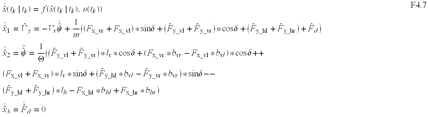
- with the estimated tire forces from the tire model, with the king pin inclinations of equation F4.6 being used.

- 4.2 Combined Yaw Rate/Sideslip Angle Control
- In the following, an embodiment of a lateral dynamics controller is described with respect to the preferred embodiment ‘Control with measured yaw rate and estimated sideslip angle’ (cf. Section 3.2 and FIG. 3). The transmission course with the controller G {dot over (ψ)} for the yaw rate component is taken from the standard ESP and will not be illustrated herein in detail.
- In FIG. 4 the essential extensions over the standard ESP are described by the part of the sideslip angle control.
- Reference Model
- In block 401 a sideslip angle reference quantity is determined as a function of the longitudinal vehicle speed x pursuant equation (F4.8):

- FIG. 6 illustrates the characteristic curve according to equation F4.8. The hatched band marks the zone of small sideslip angles of the vehicle that can still be easily mastered by the driver. No control intervention due to excessive sideslip angles is necessary within this zone |b|<|b ref |. In dependence on rising speeds, the control entry threshold is reduced to a limit value blimit,ref because large sideslip angles are more difficult for the driver to master at higher speeds.
- Typical values for the characteristic curve of the control entry threshold b ref are:
- b0,ref=7°, blimit,ref=4°, Vlimit=80km/h
- Vertical Force Model
- A stationary model pursuant equation (F4.9) is used in
block 403 for estimating the vertical forces. The vertical forces Fz are estimated with the longitudinal and lateral accelerations ax and ay applied to the center of gravity. The longitudinal acceleration may be a quantity measured by a sensor as well as a quantity estimated from the wheel speeds, e.g. in the standard ESP.
- Adaptive Torque Calculation
- In
block 404, an additional yaw torque stabilizing the vehicle is calculated according to equation (F4.11) from the sideslip angle difference - Δβ=βreƒ−{circumflex over (β)} F4.10
- in an adaptive manner, i.e., as a function of other quantities such as yaw rate {dot over (ψ)}, yaw rate control difference Δ{dot over (ψ)}, vehicle speed V x, and tire/road coefficient of friction m.

- An additional torque T req
— beta is calculated when the estimated sideslip angle {circumflex over (β)} lies outside the band limited by bref, as shown in FIG. 6. The direction of the yaw rate is another condition. When the car turns already into the ‘proper’ direction, for example {circumflex over (β)}>βreƒ and {dot over (ψ)}>0, an additional torque becomes unnecessary. No control is required below a speed Vmin. - When the conditions for an additional torque are satisfied, the additional torque is preferably calculated proportionally in relation to the deviation Db. In FIG. 7 a typical variation of the required additional torque T req
— beta in dependence on the deviation Db is shown. The zero torque T0,req— beta is necessary in order to achieve a significant additional yaw torque for driving stabilization when the control commences. However, to render the entry into the control and the exit therefrom more smoothly, it is favorable to provide a finite gradient for small deviations Db<Db0. A typical value is Db0=0.5° to 1,5°. - Further, it is suitable to increase the required additional torque T req
— beta in dependence on the frictional value m as shown in FIG. 7. - Torque Arbitration
- In
block 406 the yaw torque of the standard ESP in superposed on the yaw torque determined pursuant equation (F4.11) in the following manner: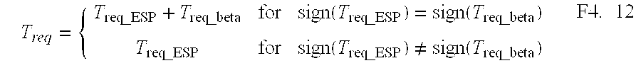
- Deactivation Logic
- The sideslip angle control is deactivated during rearward driving or when driving around a steep turn and if the difference between the king pin inclinations at the front and rear axles is large, i.e.,
- Δα=|{circumflex over (α)}v−{circumflex over (α)}h|>Δαmax F4.13
- Torque Distribution
- The nominal values of the wheel brake pressure are determined from the required additional torque in a way similar to the standard ESP. The difference compared to the standard ESP involves that with the sideslip angle control active, pressure is also required on the rear wheels in addition to the pressure requirement on the front wheels. In this respect, a distinction is made as to whether the sideslip angle control is active alone, or whether the standard ESP is active in addition.
Claims (27)
1. Method for the online determination of values of driving dynamics for a motor vehicle, characterized by the following steps:
determining estimated output quantities ŷm in dependence on determined and/or estimated input quantities u and predetermined or predicted vehicle state variables {circumflex over (x)} and optionally further quantities,
comparing the estimated output quantities ŷm with measured output quantities ŷm,
determining the estimated driving dynamics quantities {circumflex over (x)}(tk|tk) in dependence on the measurement result and, as the case may be, further criteria.
2. Method as claimed in claim 1 , characterized by the following step:
model-based determination of the predicted vehicle state variables {circumflex over (x)} in dependence on determined and/or estimated input quantities u and the driving dynamics quantities {circumflex over (x)}(tk|tk).
3. Method as claimed in claim 1 or 2, characterized in that the following input quantities u(t)={circumflex over (V)}x,δ,Fx;{circumflex over (F)}zorFz,{circumflex over (μ)}i or μi are taken into account in the estimation of the predicted vehicle state variables {circumflex over (x)} and in the determination of the driving dynamics quantities {circumflex over (x)}(tk|tk), where {circumflex over (V)}z=estimated longitudinal vehicle speed, δ=the measured steering angle, Fx=the determined longitudinal tire or wheel forces, {circumflex over (F)}z=the estimated vertical forces, or Fz=the determined vertical forces, {circumflex over (μ)}i=the estimated coefficients of friction for the tire/road contact or μi=the determined coefficients of friction for the tire/road contact.
4. Method as claimed in any one of claims 1 to 3 , characterized in that as driving dynamics quantities and the predicted vehicle state variables {circumflex over (x)}=[{circumflex over (V)}y,{circumflex over ({dot over (ψ)})}]T or {circumflex over (x)}=[{circumflex over (V)}y,{circumflex over ({dot over (ψ)})},{circumflex over (F)}d]T the lateral vehicle speed {circumflex over (V)}y, the yaw rate {circumflex over ({dot over (ψ)})} and the disturbing forces {circumflex over (F)}d, which are estimated as non-measurable input quantities, are determined.
5. Method as claimed in claim 4 , characterized in that as other quantities of driving dynamics and of the predicted vehicle state variables {circumflex over (x)}=[{circumflex over (T)}d,μi]T the disturbing torques Md and the coefficients of friction μi are determined as non-measurable input quantities.
6. Method as claimed in any one of claims 1 to 5 , characterized in that the predicted vehicle state variables {circumflex over (x)} for the next sampling moment tk+1 are achieved by integration pursuant the non-linear equation

with the start condition {circumflex over (x)}(tk|tk), where
{circumflex over (x)} estimated state vector,
f(.) continuous, non-linear system equations
x(tk) signal at the discrete moment tk. (current moment)
{circumflex over (x)}(tk|tk−1) estimated signal at the moment tk, with only information of the last moment tk−1 used
{circumflex over (x)}(tk|tk) estimated signal at the moment tk, with information of the current moment tk used
{circumflex over (x)}(tk+1|tk) predicted signal for the next moment tk+1, with only information of the current moment tk used
tk discrete moment.
7. Method as claimed in any one of claims 1 to 6 , characterized in that as an output quantity ŷm=[{circumflex over (α)}y] the lateral acceleration ay is estimated.
8. Method as claimed in claim 7 , characterized in that as another output quantity ŷm=[{dot over (ψ)}] the yaw rate {dot over (ψ)} is estimated.
9. Method as claimed in any one of claims 1 to 6 , characterized in that as still other output quantities ŷm=[{circumflex over (F)}y]T the lateral tire and wheel forces Fy. are estimated.
10. Method as claimed in any one of claims 1 to 9 , characterized in that the output quantities ŷm for the sampling moment tk are estimated according to the discrete, non-linear equation hm
ŷm(tk|tk−1)=hm({circumflex over (x)}(tk|tk−1),um(tk))
from the vehicle state variables {circumflex over (x)}(tk|tk−1) and the input quantities um(tk), where
ŷm estimated state vector of the measurable outputs
{circumflex over (x)} estimated state vector
um input vector of the measurable inputs
hm(.) discrete, non-linear measurement equations
{circumflex over (x)}(tk|tk−1) estimated signal at the moment tk, with only information of the last moment tk−1 being used
ŷ(tk|tk−1) estimated signal at the moment tk, with only information of the last moment tk−1 used
tk discrete moment.
11. Method as claimed in any one of claims 1 to 10 , characterized in that at least one of the estimated output quantities ŷm=[{circumflex over (F)}y,{circumflex over (α)}y,{circumflex over ({dot over (ψ)})}]T is compared to at least one of the determined (acquired directly or indirectly by means of sensors) output quantities ym(tk)=[Fy,αy,{dot over (ψ)}]T and the comparison results e(tk) are sent to a summation point, preferably by way of a gain matrix K, for the correction of the vehicle state variable {circumflex over (x)}(tk|tk−1), where {circumflex over (x)}(tk|tk−1)=estimated signal at the moment tk, with information of the last moment tk−1 being used.
12. Method as claimed in any one of claims 1 to 11 , characterized in that the gain matrix K at every moment tk is defined pursuant the relation K(tk)=ƒ(Â,G), where G=information content of the determined (measured) signals and Â=estimated operating point of the non-linear vehicle model.
13. Method as claimed in any one of claims 1 to 12 , characterized in that the correction of the driving dynamics quantities is carried out according to the relation
{circumflex over (x)}(tk|tk)={circumflex over (x)}(tk|tk−1)+K(tk)e(tk).
14. Method as claimed in any one of claims 1 to 13 , characterized by the step: determining the estimated controlled quantities yr at the moment tk by using information of the current moment from the driving dynamics quantities {circumflex over (x)}(tk|tk) and the input quantities um(tk) according to the relation ŷr(tk|tk−1)=hr({circumflex over (x)}(tk|tk−1),um(tk)), where um(tk)=vector of the sensed discrete input quantities.
15. Method as claimed in any one of claims 1 to 13 , characterized by the step: determining the estimated controlled quantities yr at the moment tk by using information of the last moment from the vehicle state variables {circumflex over (x)}(tk|tk−1) and the input quantities um(tk) according to the relation yr(tk|tk−1)=hr({circumflex over (x)}(tk|tk−1),um(tk)), where um(tk)=vector of the sensed discrete input quantities.
16. Method as claimed in any one of claims 1 to 15 , characterized by the steps:
determining an estimated sideslip angle {circumflex over (β)} as a controlled quantity ŷr(tk|tk−1) or ŷr(tk|tk), respectively, comparing the estimated sideslip angle {circumflex over (β)} with a sideslip angle reference quantity βreƒ, producing an additional yaw torque Treq from the estimated difference between the sideslip reference quantity βreƒ and the sideslip angle {circumflex over (β)} and a difference between a yaw rate reference quantity {dot over (ψ)}reƒ and a yaw rate {dot over (ψ)} or {circumflex over ({dot over (ψ)})} or {dot over (ψ)}linear and actuation of at least one wheel brake of the motor vehicle in dependence on the additional yaw torque Treq.
17. Method as claimed in any one of claims 1 to 16 , characterized in that the sideslip angle reference quantity βreƒ is an activation threshold that is variable in dependence on the speed Vx, e.g. Vreƒ, of the vehicle.
18. Method as claimed in any one of claims 1 to 16 , characterized in that the sideslip angle reference quantity βreƒ is determined in a dynamic model, in particular the one-track model.
19. Method as claimed in any one of claims 1 to 18 , characterized in that the yaw rate {circumflex over ({dot over (ψ)})} is estimated as a controlled quantity ŷr(tk|tk−1) or ŷr(tk|tk), respectively.
20. Method as claimed in any one of claims 1 to 19 , characterized in that the estimated yaw rate {circumflex over ({dot over (ψ)})} is produced in dependence on a measured yaw rate {dot over (ψ)} of reduced quality or a substitute signal {dot over (ψ)}linear.
21. Method as claimed in any one of claims 1 to 21 , characterized in that the additional yaw torque Treq is produced in dependence on the measured yaw rate {dot over (ψ)}.
22. Method as claimed in any one of claims 1 to 20 , characterized in that the king pin inclinations of the tires for the front axle {circumflex over (α)}v and the rear axle {circumflex over (α)}h are estimated as controlled quantity ŷr(tk|tk−1) or ŷr(tk|tk), respectively.
23. Driving dynamics control, especially ESP control or suspension control, characterized by a method as claimed in any one of claims 1 to 22 .
24. Driving dynamics control, in particular as claimed in claim 23 , characterized by a first determining unit (402) for estimating the controlled quantities {dot over (ψ)} and/or {circumflex over (α)}v, {circumflex over (α)}h from the input quantities Vx,δ,Fx,{dot over (ψ)},{circumflex over (μ)},αy,{circumflex over (F)}z, and/or, if necessary, other quantities Fz,{dot over (ψ)}linear, deactivation logic (405) for deactivating the sideslip angle control in dependence on the input quantities {circumflex over (α)}v, {circumflex over (α)}h and/or quantities representative of the driving situations of the motor vehicle, such as rearward driving, driving around a steep turn, and the like second determining unit (404) for the adaptive sideslip angle torque calculation from the input quantities
{circumflex over (β)}, βreƒ,{dot over (ψ)},Vreƒ or Vx,{circumflex over (μ)}i, respectively
third determining unit (406) for the arbitration of an additional yaw torque Treq. from the yaw torque Treg — ESP and Treg — beta.
25. Driving dynamics control as claimed in claim 23 or 24, characterized in that the first determining unit (402) is connected to a vertical force model (403) for estimating the vertical forces {circumflex over (F)}z of the motor vehicle from the input quantities αy,{circumflex over (α)}x.
26. Driving dynamics control as claimed in any one of claims 23 to 25 , characterized in that the second determining unit (404) is connected to a reference model (401) for determining the activation threshold which is variable responsive to the speed Vx or Vreƒ, respectively.
27. Use of the sideslip angle determined according to the method or in the driving dynamics control as claimed in any one of claims 1 to 26 for the purpose of active steering intervention.
Applications Claiming Priority (4)
| Application Number | Priority Date | Filing Date | Title |
|---|---|---|---|
| DE10019620 | 2000-04-19 | ||
| DE10019620.9 | 2000-04-19 | ||
| DE10046077 | 2000-09-15 | ||
| PCT/EP2001/004143 WO2001081139A1 (en) | 2000-04-19 | 2001-04-11 | Method for the online determination of values of the dynamics of vehicle movement of a motor vehicle |
Publications (2)
| Publication Number | Publication Date |
|---|---|
| US20030191572A1 true US20030191572A1 (en) | 2003-10-09 |
| US6954691B2 US6954691B2 (en) | 2005-10-11 |
Family
ID=26005401
Family Applications (1)
| Application Number | Title | Priority Date | Filing Date |
|---|---|---|---|
| US10/258,042 Expired - Fee Related US6954691B2 (en) | 2000-04-19 | 2001-04-11 | Method for determining the dynamics of vehicle movement |
Country Status (5)
| Country | Link |
|---|---|
| US (1) | US6954691B2 (en) |
| EP (1) | EP1276649B1 (en) |
| JP (1) | JP2003531066A (en) |
| DE (1) | DE10191529D2 (en) |
| WO (1) | WO2001081139A1 (en) |
Cited By (19)
| Publication number | Priority date | Publication date | Assignee | Title |
|---|---|---|---|---|
| US20040078131A1 (en) * | 2000-12-23 | 2004-04-22 | Ian Faye | Method and device for stabilizing a vehicle |
| US20040267428A1 (en) * | 2003-06-27 | 2004-12-30 | Michael Knoop | Method for coordinating a vehicle dynamics control system with an active normal force adjustment system |
| US20050004738A1 (en) * | 2001-06-28 | 2005-01-06 | Ralph Gronau | Method for modifying a driving stability control of a vehicle |
| US20060015238A1 (en) * | 2004-07-16 | 2006-01-19 | Mitsubishi Jidosha Kogyo Kabushiki Kaisha | Apparatus and method for controlling driving force supplied to wheels on opposite sides of vehicle |
| EP1623911A1 (en) * | 2004-08-04 | 2006-02-08 | Ford Global Technologies, LLC, A subsidary of Ford Motor Company | Steering System |
| US20060106516A1 (en) * | 2003-04-09 | 2006-05-18 | Pick Andrew J | Rack force disturbance rejection |
| US20060173597A1 (en) * | 2005-01-31 | 2006-08-03 | Christoph Pelchen | Method for determining a control standard of an active vehicle steering device controllable by a control device |
| US20070050112A1 (en) * | 2005-08-25 | 2007-03-01 | Robert Bosch Gmbh | Vehicle stability control system |
| US20070173997A1 (en) * | 2006-01-23 | 2007-07-26 | Nissan Motor Co., Ltd. | Sideslip angle estimation apparatus and method and automotive vehicle incorporating the same |
| US20070184929A1 (en) * | 2006-02-03 | 2007-08-09 | Jae Y. Lew | Stability-enhanced traction and yaw control using electronically controlled limited-slip differential |
| US20070193802A1 (en) * | 2006-01-31 | 2007-08-23 | Robert Bosch Gmbh | Traction control system and method |
| US20080051956A1 (en) * | 2003-12-03 | 2008-02-28 | Continental Aktiengesellschaft | Method for Controlling the Functions of an Electronic Driving Stability Program for a Motor Vehicle |
| US20080126009A1 (en) * | 2006-11-29 | 2008-05-29 | Kun-Soo Huh | Method of estimating mass of vehicle |
| US20090093924A1 (en) * | 2006-06-19 | 2009-04-09 | Toyota Jidosha Kabushiki Kaisha | Vehicle State Quantity Predicting Apparatus and Vehicle Steering Controller Using the Same, and a Method for Predicting a Vehicle State Quantity and Vehicle Steering Controlling Method Using the Same |
| US8977434B2 (en) | 2011-10-06 | 2015-03-10 | Jtekt Corporation | Vehicle attitude control system |
| US10328915B2 (en) * | 2008-01-23 | 2019-06-25 | Ford Global Tchnologies, Llc | Vehicle stability control system and method |
| CN110968088A (en) * | 2018-09-30 | 2020-04-07 | 百度(美国)有限责任公司 | Method and device for determining vehicle control parameters, vehicle-mounted controller and unmanned vehicle |
| US10997855B2 (en) * | 2018-11-07 | 2021-05-04 | Volkswagen Ag | Method and device for collecting transportation vehicle-based data records for predetermined route sections |
| US11634146B2 (en) | 2020-09-23 | 2023-04-25 | Beijing Institute Of Technology | Method and system for integrated path planning and path tracking control of autonomous vehicle |
Families Citing this family (23)
| Publication number | Priority date | Publication date | Assignee | Title |
|---|---|---|---|---|
| JP4459561B2 (en) | 2002-09-04 | 2010-04-28 | 富士重工業株式会社 | Cornering power control device and cornering power control method |
| JP2005125986A (en) * | 2003-10-27 | 2005-05-19 | Fuji Heavy Ind Ltd | Vehicle control device and vehicle control method |
| JP4268019B2 (en) * | 2003-11-14 | 2009-05-27 | 株式会社豊田中央研究所 | Body motion realizing method and apparatus |
| JP2006096230A (en) * | 2004-09-30 | 2006-04-13 | Fuji Heavy Ind Ltd | Vehicular motion control device and vehicular motion control method |
| DE102005046612B4 (en) * | 2005-09-29 | 2019-05-16 | Zf Friedrichshafen Ag | Method for realizing driving dynamics functions using a real-time tire model |
| DE102005054127A1 (en) * | 2005-11-14 | 2007-05-16 | Bosch Gmbh Robert | Method and device for controlling personal protective equipment in a rollover process |
| ATE485188T1 (en) * | 2005-12-02 | 2010-11-15 | Haldex Traction Ab | METHOD AND SYSTEM FOR VEHICLE DYNAMICS CONTROL |
| EP1798077B1 (en) * | 2005-12-16 | 2014-05-07 | Sumitomo Rubber Industries, Ltd. | Apparatus, method and program for alarming decrease in tire air-pressure |
| JP5103629B2 (en) * | 2006-02-07 | 2012-12-19 | 国立大学法人東京農工大学 | Vehicle operation measuring device and vehicle abnormal operation preventing device |
| DE102006019790A1 (en) * | 2006-04-28 | 2007-10-31 | Zf Lenksysteme Gmbh | Steering control method |
| DE102006052624A1 (en) * | 2006-11-08 | 2008-05-15 | Bayerische Motoren Werke Ag | Method for determining the lateral forces or longitudinal forces transmitted by a vehicle tire with a so-called tire model |
| DE102007013261B4 (en) * | 2007-03-20 | 2017-03-16 | Ford Global Technologies, Llc | Method and device for estimating the lateral speed of a vehicle |
| US8280591B2 (en) * | 2007-09-11 | 2012-10-02 | Bayerische Motoren Werke Aktiengesellschaft | Method for monitoring the vehicle handling of a two track vehicle |
| JP5173854B2 (en) | 2008-04-21 | 2013-04-03 | 株式会社豊田中央研究所 | Sensor drift estimation device |
| US8078373B2 (en) * | 2008-11-21 | 2011-12-13 | GM Global Technology Operations LLC | Vehicle dynamics prediction with lane/path information using a preview-correction-prediction approach |
| US8521349B2 (en) * | 2010-06-10 | 2013-08-27 | Ford Global Technologies | Vehicle steerability and stability control via independent wheel torque control |
| DE102010038971A1 (en) * | 2010-08-05 | 2012-02-09 | Robert Bosch Gmbh | Method and device for evaluating a state of a chassis of a vehicle |
| US9878738B2 (en) | 2012-03-28 | 2018-01-30 | Robert Bosch Gmbh | Non-linear compensation controller for active steering system in a vehicle |
| US10065673B2 (en) | 2012-08-02 | 2018-09-04 | Steering Solutions Ip Holding Corporation | Algorithm for tie rod force shaping |
| US8972112B2 (en) * | 2012-08-02 | 2015-03-03 | Steering Solutions Ip Holding Corporation | Algorithm for estimation of tie-rod loads |
| DE102012222884A1 (en) * | 2012-12-12 | 2014-06-12 | Robert Bosch Gmbh | Method for stabilizing a two-wheeler |
| DE102016015268B4 (en) * | 2016-12-21 | 2019-06-06 | Compagnie Générale Des Etablissements Michelin | Method for controlling a vehicle brake system for optimizing the braking process |
| US11364929B2 (en) | 2019-01-04 | 2022-06-21 | Toyota Research Institute, Inc. | Systems and methods for shared control of a vehicle |
Citations (5)
| Publication number | Priority date | Publication date | Assignee | Title |
|---|---|---|---|---|
| US5455770A (en) * | 1993-02-19 | 1995-10-03 | Robert Bosch Gmbh | Vehicle movement dynamics control system |
| US6226581B1 (en) * | 1997-06-30 | 2001-05-01 | Robert Bosch Gmbh | Method and device for controlling motion parameters representing the movement of a motor vehicle motion quantity |
| US6246945B1 (en) * | 1996-08-10 | 2001-06-12 | Daimlerchrysler Ag | Process and system for controlling the longitudinal dynamics of a motor vehicle |
| US6253123B1 (en) * | 1998-06-23 | 2001-06-26 | Robert Bosch Gmbh | Process and device for stabilizing a vehicle depending on the speed of the vehicle |
| US6604035B1 (en) * | 1998-12-29 | 2003-08-05 | Robert Bosch Gmbh | Device and method for stabilizing a vehicle |
Family Cites Families (15)
| Publication number | Priority date | Publication date | Assignee | Title |
|---|---|---|---|---|
| DE19620581B4 (en) | 1996-05-22 | 2010-06-02 | Continental Teves Ag & Co. Ohg | Device for determining the rotational behavior of a vehicle wheel |
| DE19744725A1 (en) * | 1997-10-10 | 1999-04-15 | Itt Mfg Enterprises Inc | Method to determine variable characteristics, which define motor vehicle behavior |
| US6035251A (en) | 1997-11-10 | 2000-03-07 | General Motors Corporation | Brake system control method employing yaw rate and ship angle control |
| JPH11217067A (en) * | 1997-11-27 | 1999-08-10 | Masato Abe | Calculating method of vehicle body slip angle in controlling vehicle behavior, and its device |
| US6233513B1 (en) * | 1997-11-27 | 2001-05-15 | Masato Abe | Method and system for computing a vehicle body slip angle in a vehicle movement control |
| JPH11321604A (en) * | 1998-03-17 | 1999-11-24 | Masato Abe | Calculating method of body slip angle in vehicle behavior control and device therefor |
| JPH11291929A (en) * | 1998-04-03 | 1999-10-26 | Toyota Motor Corp | Vehicle steering control device |
| JP3344648B2 (en) * | 1998-07-29 | 2002-11-11 | 株式会社豊田中央研究所 | Vehicle running state determination device |
| US6308115B1 (en) * | 1998-07-29 | 2001-10-23 | Kabushiki Kaisha Toyota Chuo Kenkyusho | Vehicle running condition judgement device |
| JP2000043616A (en) * | 1998-07-30 | 2000-02-15 | Mazda Motor Corp | Traveling control device for vehicle |
| DE59905939D1 (en) * | 1998-08-10 | 2003-07-17 | Continental Teves Ag & Co Ohg | ESP REGULATOR FOR MOTOR VEHICLES |
| JP3959860B2 (en) * | 1998-08-11 | 2007-08-15 | 日産自動車株式会社 | Vehicle body slip angle estimation method and estimation apparatus |
| JP2000062593A (en) * | 1998-08-21 | 2000-02-29 | Masato Abe | Vehicle behavior control method based on car body slip angle reference model |
| JP3817922B2 (en) * | 1998-09-04 | 2006-09-06 | トヨタ自動車株式会社 | Vehicle motion control device |
| JP3826582B2 (en) * | 1998-09-22 | 2006-09-27 | 日本精工株式会社 | Control device for electric power steering device |
-
2001
- 2001-04-11 US US10/258,042 patent/US6954691B2/en not_active Expired - Fee Related
- 2001-04-11 DE DE10191529T patent/DE10191529D2/en not_active Expired - Lifetime
- 2001-04-11 WO PCT/EP2001/004143 patent/WO2001081139A1/en active Application Filing
- 2001-04-11 EP EP01943243.4A patent/EP1276649B1/en not_active Expired - Lifetime
- 2001-04-11 JP JP2001578251A patent/JP2003531066A/en active Pending
Patent Citations (5)
| Publication number | Priority date | Publication date | Assignee | Title |
|---|---|---|---|---|
| US5455770A (en) * | 1993-02-19 | 1995-10-03 | Robert Bosch Gmbh | Vehicle movement dynamics control system |
| US6246945B1 (en) * | 1996-08-10 | 2001-06-12 | Daimlerchrysler Ag | Process and system for controlling the longitudinal dynamics of a motor vehicle |
| US6226581B1 (en) * | 1997-06-30 | 2001-05-01 | Robert Bosch Gmbh | Method and device for controlling motion parameters representing the movement of a motor vehicle motion quantity |
| US6253123B1 (en) * | 1998-06-23 | 2001-06-26 | Robert Bosch Gmbh | Process and device for stabilizing a vehicle depending on the speed of the vehicle |
| US6604035B1 (en) * | 1998-12-29 | 2003-08-05 | Robert Bosch Gmbh | Device and method for stabilizing a vehicle |
Cited By (31)
| Publication number | Priority date | Publication date | Assignee | Title |
|---|---|---|---|---|
| US6873897B2 (en) * | 2000-12-23 | 2005-03-29 | Robert Bosch Gmbh | Method and device for stabilizing a vehicle |
| US20040078131A1 (en) * | 2000-12-23 | 2004-04-22 | Ian Faye | Method and device for stabilizing a vehicle |
| US20050004738A1 (en) * | 2001-06-28 | 2005-01-06 | Ralph Gronau | Method for modifying a driving stability control of a vehicle |
| US20060106516A1 (en) * | 2003-04-09 | 2006-05-18 | Pick Andrew J | Rack force disturbance rejection |
| US7273127B2 (en) | 2003-04-09 | 2007-09-25 | Trw Limited | Rack force disturbance rejection |
| US20040267428A1 (en) * | 2003-06-27 | 2004-12-30 | Michael Knoop | Method for coordinating a vehicle dynamics control system with an active normal force adjustment system |
| US7308351B2 (en) * | 2003-06-27 | 2007-12-11 | Robert Bosch Gmbh | Method for coordinating a vehicle dynamics control system with an active normal force adjustment system |
| US7937205B2 (en) * | 2003-12-03 | 2011-05-03 | Continental Aktiengesellschaft | Method for controlling the functions of an electronic driving stability program for a motor vehicle |
| US20080051956A1 (en) * | 2003-12-03 | 2008-02-28 | Continental Aktiengesellschaft | Method for Controlling the Functions of an Electronic Driving Stability Program for a Motor Vehicle |
| US7263424B2 (en) * | 2004-07-16 | 2007-08-28 | Mitsubishi Jidosha Kogyo Kabushiki Kaisha | Apparatus and method for controlling driving force supplied to wheels on opposite sides of vehicle |
| US20060015238A1 (en) * | 2004-07-16 | 2006-01-19 | Mitsubishi Jidosha Kogyo Kabushiki Kaisha | Apparatus and method for controlling driving force supplied to wheels on opposite sides of vehicle |
| EP1623911A1 (en) * | 2004-08-04 | 2006-02-08 | Ford Global Technologies, LLC, A subsidary of Ford Motor Company | Steering System |
| US20060173597A1 (en) * | 2005-01-31 | 2006-08-03 | Christoph Pelchen | Method for determining a control standard of an active vehicle steering device controllable by a control device |
| US7418327B2 (en) * | 2005-01-31 | 2008-08-26 | Zf Friedrichshafen Ag | Method for determining a control standard of an active vehicle steering device controllable by a control device |
| US7966113B2 (en) * | 2005-08-25 | 2011-06-21 | Robert Bosch Gmbh | Vehicle stability control system |
| US20070050112A1 (en) * | 2005-08-25 | 2007-03-01 | Robert Bosch Gmbh | Vehicle stability control system |
| US20070173997A1 (en) * | 2006-01-23 | 2007-07-26 | Nissan Motor Co., Ltd. | Sideslip angle estimation apparatus and method and automotive vehicle incorporating the same |
| US7844383B2 (en) * | 2006-01-23 | 2010-11-30 | Nissan Motor Co., Ltd. | Sideslip angle estimation apparatus and method and automotive vehicle incorporating the same |
| US7641014B2 (en) | 2006-01-31 | 2010-01-05 | Robert Bosch Gmbh | Traction control system and method |
| US20070193802A1 (en) * | 2006-01-31 | 2007-08-23 | Robert Bosch Gmbh | Traction control system and method |
| US7801657B2 (en) * | 2006-02-03 | 2010-09-21 | Eaton Corporation | Stability-enhanced traction and yaw control using electronically controlled limited-slip differential |
| US20070184929A1 (en) * | 2006-02-03 | 2007-08-09 | Jae Y. Lew | Stability-enhanced traction and yaw control using electronically controlled limited-slip differential |
| US20090093924A1 (en) * | 2006-06-19 | 2009-04-09 | Toyota Jidosha Kabushiki Kaisha | Vehicle State Quantity Predicting Apparatus and Vehicle Steering Controller Using the Same, and a Method for Predicting a Vehicle State Quantity and Vehicle Steering Controlling Method Using the Same |
| US8090493B2 (en) * | 2006-06-19 | 2012-01-03 | Toyota Jidosha Kabushiki Kaisha | Vehicle state quantity predicting apparatus and vehicle steering controller using the same, and a method for predicting a vehicle state quantity and vehicle steering controlling method using the same |
| US7499826B2 (en) * | 2006-11-29 | 2009-03-03 | Hyundai Motor Company | Method of estimating mass for vehicle safety |
| US20080126009A1 (en) * | 2006-11-29 | 2008-05-29 | Kun-Soo Huh | Method of estimating mass of vehicle |
| US10328915B2 (en) * | 2008-01-23 | 2019-06-25 | Ford Global Tchnologies, Llc | Vehicle stability control system and method |
| US8977434B2 (en) | 2011-10-06 | 2015-03-10 | Jtekt Corporation | Vehicle attitude control system |
| CN110968088A (en) * | 2018-09-30 | 2020-04-07 | 百度(美国)有限责任公司 | Method and device for determining vehicle control parameters, vehicle-mounted controller and unmanned vehicle |
| US10997855B2 (en) * | 2018-11-07 | 2021-05-04 | Volkswagen Ag | Method and device for collecting transportation vehicle-based data records for predetermined route sections |
| US11634146B2 (en) | 2020-09-23 | 2023-04-25 | Beijing Institute Of Technology | Method and system for integrated path planning and path tracking control of autonomous vehicle |
Also Published As
| Publication number | Publication date |
|---|---|
| WO2001081139A8 (en) | 2001-11-22 |
| EP1276649A1 (en) | 2003-01-22 |
| US6954691B2 (en) | 2005-10-11 |
| DE10191529D2 (en) | 2004-07-08 |
| JP2003531066A (en) | 2003-10-21 |
| EP1276649B1 (en) | 2015-08-05 |
| WO2001081139A1 (en) | 2001-11-01 |
Similar Documents
| Publication | Publication Date | Title |
|---|---|---|
| US6954691B2 (en) | Method for determining the dynamics of vehicle movement | |
| US8073608B2 (en) | Yaw stability control system | |
| US6895318B1 (en) | Oversteer steering assistance controller | |
| US6941213B2 (en) | Road condition estimation apparatus | |
| US7308351B2 (en) | Method for coordinating a vehicle dynamics control system with an active normal force adjustment system | |
| US6862512B2 (en) | Method and system for controlling the performance of a motor vehicle | |
| US8200392B2 (en) | Vehicular steering control device | |
| US20050102085A1 (en) | Stability factor learning method and apparatus for a vehicle and control apparatus for a vehicle | |
| US20070173997A1 (en) | Sideslip angle estimation apparatus and method and automotive vehicle incorporating the same | |
| JP3970095B2 (en) | Steering device | |
| EP1760451A1 (en) | Method and system for road surface friction coefficient estimation | |
| US8712641B2 (en) | Stability control system with body-force-disturbance heading correction | |
| US6169951B1 (en) | Active brake control having yaw rate estimation | |
| JP3424192B2 (en) | Automotive control method and device | |
| US8548681B2 (en) | Power steering device | |
| US6560524B2 (en) | Integration of rear wheel steering with vehicle stability enhancement system | |
| JP2005511399A (en) | Apparatus and method for determining parameters affected by vehicle vehicle dynamics | |
| JP3882894B2 (en) | Steering reaction force control device | |
| JP2006501094A (en) | Method for determining steering torque | |
| JP2006501094A5 (en) | ||
| JP2007240392A (en) | Ground load estimation device | |
| JP3039071B2 (en) | Vehicle turning limit judgment device | |
| JP5089558B2 (en) | Road friction coefficient estimation device | |
| CN114379288A (en) | Method for early detection of irregular wear of motor vehicle tyres and/or unintentional changes in chassis settings | |
| JP4630039B2 (en) | Vehicle steering control device |
Legal Events
| Date | Code | Title | Description |
|---|---|---|---|
| AS | Assignment |
Owner name: CONTINENTAL TEVES AG & CO. OHG, GERMANY Free format text: ASSIGNMENT OF ASSIGNORS INTEREST;ASSIGNORS:ROLL, GEORG;LUDERS, ULRICH;OEHLER, RAINER;AND OTHERS;REEL/FRAME:014232/0393 Effective date: 20021023 |
|
| REMI | Maintenance fee reminder mailed | ||
| LAPS | Lapse for failure to pay maintenance fees | ||
| STCH | Information on status: patent discontinuation |
Free format text: PATENT EXPIRED DUE TO NONPAYMENT OF MAINTENANCE FEES UNDER 37 CFR 1.362 |
|
| FP | Lapsed due to failure to pay maintenance fee |
Effective date: 20091011 |