US4893262A - Weigh feeding system with self-tuning stochastic control - Google Patents

Abstract

A weigh feeding system using a stochastic controller wherein the weight of material is sensed, and an estimate of the mass flow state of the material being discharged is created by use of a Kalman filter process. Plant noise processes and measurement noise processes, which affect the measured weight signal, are modeled as stochastic processes and are used, in combination with the sensed weight signal, to calculate the estimated mass flow state. The noise model is modified to account for disturbances. The estimated mass flow state signal is used to calculate a motor feedback signal which, in turn, is used to control the speed of the discharge apparatus. In this manner, the mass flow of the material actually being discharged is driven to a desired mass flow with minimum error variance in the presence of unavoidable plant and measurement noise. Self-tuning of the stochastic controller is employed to accurately determine parameters of the plant noise and measurement noise processes, and to compensate the controller for control dynamics. Feedback control tuning is also employed to monitor the set-point error in order to achieve quick response while maintaining smooth steady-state set point control.

Description

This application is a continuation of application Ser. No. 174,976, filed Mar. 29, 1988 and now abandoned, which is a continuation-in-part of Application Ser. No. 879,430, filed June 27, 1986, now U.S. Pat. No. 4,775,949.

A portion of the disclosure of this patent document contains material which is subject to copyright protection. The copyright owner has no objection to the facsimile reproduction by anyone of the patent document or the patent disclosure, as it appears in the Patent and Trademark Office patent file or records, but otherwise reserves all copyright rights whatsoever.

This invention pertains to weight feeding systems.

The present invention uses a Kalman filtering process to develop filtered estimates of the actual weight state and the mass flow state. These filtered estimates are used, in combination with modeling and classification of the plant and measurement noise processes which affect the weight measurements, to control the actual mass flow state. The class of noise is determined, and a stochastic model for each class is created. The estimated mass flow signal is produced based on the measured weight and the stochastic models of the individual noise processes affecting the system. The noise process models are modified according to the magnitude of their effects and probability of occurrence.

The estimated mass flow state signal is then compared with a desired mass flow set-point, and the resultant error signal is used to control a discharge actuator to produce the desired mass flow.

The present invention also employs self-tuning of parameters associated with the noise processes which affect the weight measurements and self-tuning of control parameters in order to compensate the Kalman filter states due to the effects of control dynamics. This noise model tuning and control model tuning allow the Kalman filter to operate optimally. In addition, feedback control tuning is employed to monitor the set point error and to generate adaptive dynamics to achieve a quick response while maintaining a smooth steady-state set point control.

BRIEF DESCRIPTION OF THE DRAWINGS

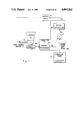
FIG. 1 is a loss-in-weight feeding system embodying the present invention.

FIG. 2 is a schematic of a model of a discrete-time loss-in-weight system.

FIG. 3 is a schematic of a model of a discrete-time loss-in-weight system, a Kalman filter to estimate mass flow and a motor control signal processor according to the present invention.

FIGS. 4A-4C are flowcharts of the computational steps performed by the weight signal processor of the present invention.

FIG. 5 is a flowchart of the computational steps performed by the motor controller of the present invention.

FIGS. 6A-4F are graphs of the operation of a weigh feeding system according to the present invention.

FIG. 7 is a tubular representation of the graphs of FIGS. 6D and 6E.

FIG. 8 is another graph of the operation of a weigh feeding system according to the present invention.

FIG. 9 is a loss-in-weight feeding system including self-tuning and embodying the present invention.

FIG. 10 is a flowchart of computational steps performed by the weight signal processor of the present invention employing self-tunning.

FIG. 11 is a flowchart of the computational steps performed by the motor controller of the present invention employing self-tuning.

FIG. 12 is a flowchart of the computational steps performed by the present invention to calibrate control parameters.

FIG. 13 is a schematic of a model of the noise parameter calibration of the present invention.

FIG. 14 is a flowchart of the computational steps performed by the present invention to calibrate noise parameters.

DESCRIPTION OF THE PREFERRED EMBODIMENT

In the present weight feeding system, solid or liquid material stored in a hopper or other container is discharged by a conventional discharge actuator such as a screw feeder, conveyor, pump, valve or the like as appropriate. The discharge actuator is driven by an electric motor. The system also includes a weight sensing device, such as a scale, for sensing the weight of the material in the hopper or the material being discharged, and for producing a signal indicative of the sensed weight state. The signal produced by the weight sensing device is applied to a weight signal processor which, in turn, produces a signal which is an estimate of the weight rate state or mass flow state of material being discharged. The estimate of mass flow state is then used, in a feedback loop, to control the motor to drive the estimated mass flow state to a desired set-point mass flow.

Referring to FIG. 1, material stored in hopper 10 is discharged by feed screw 11 driven by feed screw motor 12. Scale 13 measures the combined weight of hopper 10 feed screw 11 and motor 12 to produce a measured weight signal W_m. It will be understood that in a conveyer weigh feeder, scale 13 would sense the weight of material being discharged upon at least a portion of the length of the conveyer. Signal W_m is applied to weight signal processor 14 in computer 15 which produces an estimate, W_r, of the mass flow state of material based upon the measured weight W_m. An operator enters a desired mass flow set-point W_rd through control panel 16. The estimated mass flow state W_r is compared with the desired mass flow W_rd by summing junction 17 to produce an error signal state W_re. The error signal state is used by motor controller 18 to calculate a motor control signal I_M which is applied to motor drive 19. The estimated mass flow state W_r, and the actual mass flow, are thus driven to the desired set-point W_rd.

The weight sensor is, of course, subject to random and systematic instrument and phenomenon errors. The sensor produces erroneous results not only because of internal electronic noise, but also because of the physical inertia of the sensor as well as effects of external electronic noise.

In addition, the physical plant including the material hopper, feed screw and motor are also susceptible of disturbance. These plant disturbance processes include: vibrational noise due to the mechanical movement of the feeding screw or material mixer contained within the hopper; varying or non-uniform output feed due to lumpy material or non-uniform screw discharge; refilling of the hopper with material at times and at refill rates that are uncertain; unintentional aperiodic superimposed hopper disturbances such as bumping the feeder, or dropping or lifting extraneous weights such as tools; and periodic and aperiodic disturbances of the hopper due to environmental effects such as wind, neighboring machines or passing vehicles.

In general then, a weight measurement yields only crude information about a loss-in-weight feeding system's behavior and, by itself, may be unsatisfactory for assessing the system's states and ultimately controlling the mass flow.

The mathematical model of a discrete-time material discharge system is shown in FIG. 2. The actual weight state of material at time k+1 is produced by summing junction 21 which provides the sum of the actual weight state at time k, W(k), the plant noise process affecting the weight at time k, w₁ (k), the effect of the motor control on the weight, u₁ (k), and the actual mass flow state at time k, W_r (k), multiplied by the sampling time T. This multiplication by T represents a time integration of mass flow state, W_r. Actual weight state signal W(k+1) is applied to delay block 22 to produce actual weight state signal W(k). The measured weight signal W_m (k) is produced by summing junction 23 which adds measurement noise process n(k) to actual weight state signal W(k).

The actual mass flow state at time k+1, W_r (k+1), is produced by summing junction 24 which provides the sum of the actual mass flow state at time k, W_r (k), the effect of the motor control on the mass flow, u₂ (k), and the mass flow plant noise process w₂ (k). The mass flow state at time k, W_r (k) is produced from the actual mass flow state W_r (k+1) via delay block 26.

The block diagram of FIG. 2 is a schematic representation of the following mathematical equations:

W(k+1)=W(k)+TW.sub.r (k)+u.sub.1 (k)+w.sub.1 (k)

W.sub.r (k+1)=W.sub.r (k)+u.sub.2 (k)+w.sub.2 (k)

W.sub.m (k)=W(k)+n(k)

where:

k=1, 2, 3, . . .

W(k) is the actual weight state at time k;

W_r (k) is the actual mass flow state at time k;

W_m (k) is the weight measurement at time k;

T is the time period between samples;

u₁ (k) is the effect of the motor control on the actual weight state;

u₂ (k) is the effect of the motor control on the actual mass flow state;

n(k) is the measurement noise;

w₁ (k) is the plant weight noise perturbation; and

w₂ (k) is the plant mass flow noise perturbation.

Weight state W and mass flow state W_r are known as state variables, and the mass flow state is the time derivative of the weight state (i.e., the weight is the integral of the mass flow). The only state variable sensed is the weight W which can only be sensed indirectly from the noise corrupted signal W_m. It is to be noted that noise processes n, w₁ and w₂ are unavoidable and are always present in the system. Controlling, via u₁ and u₂, the discharge using only measured weight signal W_m in ignorance of the plant and measurement noise processes, will invariably result in an inferior system.

FIG. 3 is a block diagram of a real discrete-time material discharge system connected to a block diagram of a discrete-time weight signal processor and motor controller according to the present invention. Elements identical to those in FIGS. 1 and 2 bear the same numeral identifier. The weight signal processor uses a Kalman filtering process to develop a filtered estimate of the actual weight state W(k) and a filtered estimate of the mass flow state W_r (k). The estimate of mass flow state W_r (k) is used, by motor controller 18, as shown schematically in FIG. 3 and in detail in FIGS. 5 and 11, to calculate motor control signal I_M and motor controls u₁ (k) and u₂ (k). Motor controls u₁ (k) and u₂ (k) are the mathematical affects on actual weight state W(k) and actual mass flow state W_r (k), respectively, and are used in the prediction process of estimated weight state W(k) and estimated mass flow state W_r (k).

In the lower portion of FIG. 3 is signal processor 14, summing junction 17 and motor controller 18 shown in FIG. 1. The signal processor is configured as a Kalman filter whose structure is identical to the mathematical model of the real system. Summing junctions 27 and 28 perform the function of summing junctions 21 and 24 in the real system. Delay blocks 29 and 31 model the functions of real delay blocks 22 and 26, respectively.

Summing junction 32 provides the difference between measured weight W_m (k) and estimated weight state W(k). This difference, W_m (k), also known as the measurement residual, is multiplied by gain K_W (k) and applied to summing junction 27 in calculating the next weight state estimate W(k+1). W_m (k) is also multiplied by gain K_W.sbsb.r (k) and applied to summing junction 28 in calculating the next mass flow state estimate W_r (k+1). Gains K_W and K_W.sbsb.r are known as the Kalman gains and are variable according to the error covariance of the estimated weight state W and estimated mass flow state W_r relative to the real values of W and W_r, while taking into account noise processes n, w₁ and w₂. Details of the calculation of Kalman gains K_W and K_W.sbsb.r are presented below referring to FIG. 4.

Since the effects of the noise processes n, w₁ and w₂ are used in the calculation of the Kalman gains, it is important not only to identify the various noise sources and their effect on the state variables W and W_r, but also to model their magnitudes and to include the magnitudes into the Kalman gain calculation.

Each noise process is modeled as a zero mean, white process with the following noise covariances: ##EQU1## where: .sub.σ 2_n is the variance of the measurement noise process;

.sub.σ 2_w1 is the variance of the plant noise process affecting the weight;

.sub.σ 2_w2 is the variance of the plant noise process affecting the mass flow; and

.sub.σ 2_w1,w2 is the covariance of plant noise processes w₁ and w₂.

As mentioned above, plant noise processes w₁ and w₂ are the weight noise perturbation and mass flow noise perturbation, respectively. In a practical system, mass flow noise perturbation w₂ is a regular noise process due to, for example, lumpy or non-uniform material being fed. Weight noise perturbation w₁ is an irregular process due to highly unpredictable sources, such as vibrations from passing vehicles, or physical impact with the material hopper. Measurement noise process n is also a regular noise process due to random and systematic measurement instrument and discharge system phenomenon errors. For example, vibrations from the feed screw or material mixer, in addition to weight sensor inaccuracies, contribute to measurement noise process n.

Variance, σ² n can be determined experimentally or emperically from an actual system. For example, the material discharge system may be operated without loss in weight and variance σ² n can be calculted from a series of weight measurements W_m (k). The variance, σ² w₂, can be calculated from machine operational specifications. For example, if the desired mass flow deviation (σ_W.sbsb.d) is specified, σ_w.sbsb.2 can be set proportional to σ_W.sbsb.d. In the preferred alternate embodiment, variances σ² _n and σ² _w.sbsb.2 are calculated using a self-tuning procedure described in detail below with reference to FIGS. 9-14.

In contrast, plant noise process w₁, being unpredictable, is modeled as having variance A, where A is determined from the magnitude of the sensed measurement residual. Details of this process and calculation of A are described below with reference to FIG. 4B.

Finally, since the plant noise processes are typically not correlated, σ² _w.sbsb.1,_w.sbsb.2 is equal to 0.

The plant noise covariance matrix Q(k) is determined in the following manner. First, Q(k) is set equal to Q_o. where: ##EQU2## Next, A is calculated from the magnitude of the measurement residual and the probability of occurrence of that magnitude of residual. Then Q(k) is replaced by Q₁ where: ##EQU3##

Referring to FIGS. 4A-4C, the process steps executed by signal processor 14 (FIG. 1) are shown. After the process is started, the following parameters are initialized in step 41.

W_rd --the desire mass flow set point;

σn--the standard deviation of measurement noise n;

σw_d --the desired standard deviation of mass flow;

T--the weight signal (W_m) sampling period;

G--the gain constant of the motor controller;

τ_m --the time constant of the screw motor;

T_d --the commutation delay associated with the feed motor; and

FF--the feed factor of the feed screw motor.

In Step 42, the variance, σ² _w.sbsb.2, is calculated from the desired standard deviation of mass flow, σ_w.sbsb.d. This is an iterative calculation based on the known steady state relationship between the desired mass flow error variance (σ² w_r ⁼ σ² w_d) and the parameters T, σ² n and σ² w₂. The iterative calculation is shown in the routine spanning lines 4999-5220 of the source code listing without self-tuning submitted herewith. In the preferred alternate embodiment, self-tuning is employed to calculate both estimated noise variances σ² _n and σ² _w.sbsb.2, using the self-tuning procedure described in detail below with reference to FIGS. 9-14. In step 43 the following variables are all initially set to 0:

W_cp --weight control signal;

u₁, u₂ --motor controls affecting weight and mass flow, respectively.

Also in step 43, feed screw motor signal, I_M, is initialized at a desired level so that the motor is initially moving at a desired speed. In the alternative, signal I_M may be initialized to 0 so that the motor is initially stationary.

In step 44, counter k is set to 0, and control is transferred to step 45 where the first weight sample W_m (1) is taken. Control is then transferred to decision block 46 where, if k+1 is greater than 2, indicating that the filter has already been initialized, control is transferred to the process steps of FIG. 4B. Otherwise, control is transferred to decision block 47 where, if k+1 is not equal to 2, control is transferred to block 48 and counter k is incremented. Another weight sample is then taken in block 45. If decision block 47 decides that k+1 is equal to 2, control is transferred to block 49 where filter initialization is begun.

In block 49, the initial weight state estimate, W, is set to the measured weight at time k=2. In addition, the initial mass flow state estimate, W_r, is set to the difference between the first two weight measurements divided by sampling period T. Thus, the initial estimates for weight and mass flow states are found using the last weight signal and its simple time derivative. Also in block 49, the predicted estimate of weight state at time k=3 is set to the estimated weight state at time k=2 plus T times the estimated mass flow state at time k=2, and the predicted estimate of mass flow state at time k=3 is set to the estimated mass flow state at time k=2.

After the extimates and predictions of weight and mass flow states are initialized in block 49, control is transferred to block 51 where the four entries of the error covariance matrix P are initialized.

The error covariance matrix P takes the form: ##EQU4## where: σ² _W is the variance of the weight error;

σ² _W.sbsb.r is the variance of the mass flow error; and

σ² _W,W.sbsb.r is the covariance of the weight and mass flow errors.

After error covariance matrix P is initialized in block 51, control is transferred to block 48 where counter k is incremented and another weight sample is taken in block 45. Once the filter is initialized, k+1 will be greater than 2 and decision block 46 will transfer control to block 56 of FIG. 4B.

When self-tuning is employed, the process steps shown in the flow chart of FIG. 10, described in detail later, are employed instead of those shown in FIG. 4A.

In block 56, plant noise covariance matrix Q(k) is set to Q₀ and control is transferred to block 57 where error covariance matrix P is updated using the matrix equation:

P(K+1|k)=FP(k|k)F'+Q(k)

where:

P(k+1|k) is the prediction of error covariance matrix P at time k+1 given measurements up to and including time k;

P(k|k) is the error covariance matrix P at time k given measurements up to and including time k; ##EQU5## F' is the transpose of F; and Q(k) is the plant noise covariance matrix at time k.

It should be noted that the diagonal elements of the P matrix (σ² _W and σ² _W.sbsb.r) are a measure of the performance of the estimation process. Although theoretically impossible, if the variance of the weight error σ² _W, and the variance of the mass flow error, σ² _W.sbsb.r, are both zero, the estimates are perfect, i.e., the same as the real states. As a practical matter, only minimization of these error variances is realizable.

Control is then transferred to block 58 where the measurement residual is calculated using the equation:

W.sub.m (k+1|k)=W.sub.m (k+1)-W(k+1|k)

where:

W_m (k+1|k) is the measurement residual at time k+1 given measurements up to and including time k;

W_m (k+1) is the weight measurement at time k+1; and

W(k+1|k) is the estimated weight state at time k+1 given measurements up to and including time k.

Control is then transferred to block 59 where the measurement residual variance is calculated using the matrix equation:

σ.sup.2.sub.W.sbsb.m =HP(k+1|k)H'+R(k+1)

where:

H=[10];

H' is the transpose of H;

P(k+1|k) is calculated in block 57; and

R(k+1) is the measurement noise variance at time k+1 (actually σ² n).

Control then passes to decision block 60 where flag j is tested to decide if, during the present cycle, variance A has already been calculated by traversing the loop shown in FIG. 4B. If variance A has not yet been calculated this cycle, control is transferred to block 61 where variable x is set to the measurement residual W_m (k+1|k) divided by a constant q and the standard deviation of the measurement residual (the square root of the variance calculated in block 59). Constant q is preferably in the range of 3≦q≦5, however, values outside of this range are acceptable without departing from the scope of the invention.

An adaptive distribution function f(x) is also calculated in block 61 by the equation:

f(x)=|x|.sup.a /(b+|x|.sup.a)

where:

2≦a≦4.

Values outside of this range are acceptable without departing from the scope of the invention. The exact values of q and a depend upon the particular weigh feeder used and are determined experimentally in order to minimize the various elements of the error covariance matrix P during normal operation, and to minimize the deletarious effects of aperiodic hopper disturbance (such as refill).

f(x) represents the probability that the cause of the present measurement residual is a source outside of that indicated by the previous error covariance matrix P(k+1|k) (calculated in block 57), and due to measurement noise n(k) and mass flow noise w₂ (k).

Control then passes to block 62 where variance A is calculated as the product of the adaptive distribution function, f(x), multiplied by the square of the measurement residual divided by 12. This results in a uniform distribution for A.

Control then passes to block 63 where matrix Q(k) is set equal to Q₁, and flag j is set equal to 1 in block 64 before returning control to block 57.

Then, using the new value for Q(k), the error covariance matrix is recalculated in block 57, the measurement residual is recalculated in block 58 and the measurement residual variance is recalculated in block 59. Next, since flag j is now 1, control passes from block 60 to block 65 where counter j is reset to 0. Control is then transferred to block 66 of FIG. 4C.

Referring to FIG. 4C, the filter gains K are calculated in block 66 using the matrix equation:

K(k+1)=P(k+1|k)H'[HP(k+1|k)H'+R(k+1)].sup.-1

where: ##EQU6## K_w (k+1) is the weight Kalman gain at time k+1; K_w.sbsb.r (k+1) is the mass flow Kalman gain at time k+1; and

all other variables have been previously defined or calculated.

The predicted weight state W and predicted mass flow state W_r, at time k+1 given measurements up to and including time k+1, are then calculated in block 67 using the equations:

W(k+1|k+1)=W(k+1|k)+K.sub.w (k+1)W.sub.m (k+1|k)

W.sub.r (k+1|k+1)=W.sub.r (k+1|k)+K.sub.w.sbsb.r (k+1)W.sub.m (k+1|k)

where all variables have been previously defined and calculated.

Control is then transferred to block 68 where error covariance matrix P is updated. The matrix I appearing in the equation in block 68 is the identity matrix. All other variables have been previously defined and calculated.

Control is then transferred to block 69 where new predictions for estimated weight state W and mass flow state W_r are calculated for time k+2 given measurements up to and including time k+1, using the following equations:

W(k+2|k+1)=W(k+1|k+1)+TW.sub.r (k+1|k+1)+u.sub.1 (k+1)

W.sub.r (k+2|k+1)=W.sub.r (k+1|k+1)+u.sub.2 (k+1)

where:

u₁ (k+1) is the value of the motor control applied at time k+1 which is predicted to affect the weight state at time k+2;

u₂ (k+1) is the value of the motor control applied at time k+1 which is predicted to affect the mass flow state at time k+2; and

where all other variables have been previously defined and calculated.

Control is then transferred to block 71 where the motor control is updated. The details of the processing steps performed within block 71 are shown in FIG. 5.

Upon exiting block 71, control is returned to block 48 (FIG. 4A) where counter k is incremented and the entire loop is retraced. It should be noted that, since the time necessary to traverse the loop may vary slightly from cycle to cycle, sampling period T is changed slightly from period to period. In the preferred embodiment, T is in the range of 0.75≦T≦2.0 seconds although time periods outside of this range also produce acceptable results. Recalculation of T each cycle is illustrated in FIG. 6F.

Referring to FIG. 5, in block 72, mass flow error signal, W_re, is calculated as the difference between desired mass flow set point, W_rd, and the mass flow state estimate, W_r, previously calculated in block 69 of FIG. 4C. Control is then transferred to block 73 where weight rate control signal, W_rc, is calculated as the product of gain, G, and mass flow error, W_re. Motor signal I_M is then adjusted by weight rate control signal, W_rc, divided by feed factor FF. Feed factor FF is used to convert the mass flow state variable to the motor speed signal in order to compensate for the nonlinear relationship between motor signal I_M and motor speed.

Control is then transferred to block 74 where motor controls u₁ and u₂, are calculated. These calculations represent a model of the control portion of the material discharge system. This is to be distinguished from the model of the estimation or filtering shown in FIG. 3 and in the process steps of FIGS. 4A-4C.

In block 76, past weight control signal, W_cp, is set equal to the weight control signal just calculated, W_rc.

In step 77, caculated motor signal, I_M, is output to a motor controller to control the rate of the material discharge.

It should be emphasized that the Kalman filter process of the present invention is a recursive process which requires very little information be stored and carried over from one calculation time interval to the next. Therefore, the present invention can be readily adapted for use in existing material discharge systems by reprogramming microprocessor program memories, and by using preexisting random access memories.

An alternative preferred embodiment of motor control calculations employing self-tuning procedures is shown in the flow chart of FIG. 11, described in detail later.

FIGS. 6A-6F graphically illustrate the operation of an actual weigh feeding system under closed-loop computer control.

The system was started at cycle 0 with the following initial parameters: T=1.3; W_rd =500; FF=0.3; q=3; and a =2. The system was started and run for approximately 100 calculation cycles while feeding semolina. Both natural plant and measurement noise were present. In addition, the system hopper was subjected to the following deliberate outside perturbations:

______________________________________                                    
Approximate                                                               
Cycle Time        Perturbation                                            
______________________________________                                    
25                17 mm wrench on                                         
35                17 mm wrench off                                        
55                3 Kg weight on                                          
65                3 Kg weight off                                         
90                Material refill                                         
______________________________________                                    

The ordinate in graphs 6A-6C is in parts per million where one million parts is equal to approximately 150 Kg (the maximum measurable weight of the weight sensor used). In other words, a reading of 600,000 parts per million equals 60% of 150 Kg, or 90 Kg.

In FIG. 6D, the units of motor signal I_M are directly convertable to a motor drive signal, for example, a frequency. The units of mass flow estimate in FIG. 6E are in parts per million per unit time and are directly convertable to Kg/sec.

FIG. 6F illustrates the variability of sample period T from one cycle to the next.

FIG. 7 is a tabular presentation of the graphs of FIGS. 6D and 6E.

FIG. 8 is a graphical display of the same system as that operated to produce the graphs of FIGS. 6A-6F, showing operation with only the natural plant and measurement noise processes present without any outside perturbations.

The following is a commented source code listing of a computer program for computer 15 of the preferred embodiment. This program incorporates the steps shown in the flowcharts of FIGS. 4A-4C and 5. ##SPC1##

In order to facilitate the calculation of the various operational parameters, self-tuning is used to control the feeding process to generate data from which these various operational parameters can be calculated. FIG. 9 is similar to FIG. 1, and illustrates a conceptual block diagram of the general self-tuning process used to generate data from which the stochastic control and noise parameters are calculated. Functional blocks identical to those of FIG. 1 bear identical numeral designators and will not be described again.

In the general self-tuning process of the present invention, when a weigh feeding machine is first started, or when a dramatic change in operating conditions is presented (for example, changing the type of material being fed), the feeding machine is set to a calibration or tune mode shown schematically by switch 81. In the calibration mode, system calibration processer and control generator 82 causes a series of control signals u(k) to be applied to the weigh feeder, and the weigh feeder reacts to the control sequence u(k). Weight sensor 13 generates a corresponding measurement sequence z(k). the input/output signals (u(k) and z(k)) are then used by the system calibration processor and control generator 82 to estimate the noise and control parameters, for example. Then, the estimated parameters are sent to the Kalman filter, the calibration mode is exited and closed-loop control begins.

The calibration process is performed when the system is started, or whenever recalibration is desired by the system operator. FIG. 10 is similar to FIG. 4A and includes self-tuning procedures. Functional blocks in FIG. 10 which are identical to those of FIG. 4A bear identical numeral designators.

Refering to FIG. 10, after the system is started, the following parameters are initialized in step 83:

W_rd --the desire mass flow set point;

σ_n --the standard deviation of measurement noise n;

σ_w.sbsb.2 --the standard deviation of mass flow noise;

T--the weight signal (W_m) sampling period;

G_c --the gain constant of the motor controller;

FF--the feed factor of the feed screw motor; and

A--the magnitude of the square wave used to calibrate control parameters (discussed in detail below with reference to FIG. 12).

The standard deviations for measurement noise σ_n and mass flow noise σ_w.sbsb.2 are either carried over from previous machine operation (for example, parameters calculated during a previous factory shift, or the like), or are entered and/or calculated as described above with reference to FIG. 4A.

Control then passes to decision block 84 where it is decided, under operator control, whether the controller should be calibrated. If not, for example, if the various parameters had been calibrated during an earlier operating period of the weigh feeding machine, control is transferred directly to block 43, and control proceeds as described above with reference to FIGS. 4A-C. If calibration is desired, for example, if the type of material being fed is changed, control is transferred to blocks 86 and 87 where the control parameters, GV_ss and W_cf, and noise parameters, σ_n and σ_w.sbsb.2, are respectively calibrated using the procedures depicted in FIGS. 12 and 14, described in detail below.

After parameter calibration in blocks 86 and 87, control passes to block 43, and proceeds as described above with reference to FIGS. 4A-C.

In this alternate preferred embodiment, when motor control is calculated in block 71 of FIG. 4C, the adaptive motor control calculations shown in FIG. 11 are performed.

Referring to FIG. 11, in block 88, the predicted set-point error, W_re (k+1|k), is calculated using the equation:

W.sub.re (k+1|k)=W.sub.rd -[W.sub.r (k|k)+GV.sub.ss W.sub.rc (k-1)]

where:

W_re (k+1|k) is the predicted set-point error for time k+1 given measurements up to and including time k;

W_rd is the desired set-point;

W_r (k|k) is the estimated mass flow state at time k given measurements up to and including time k;

GV_ss is the small signal gain; and

W_rc (k-1) is the weight rate control signal calculated the previous cycle.

Small signal gain GV_ss is calibrated during the control calibration process described below with refernce to FIG. 12.

Control then passes to decision block 89 where the predicted set-point error, W_re (k+1|k), calculated in block 88 is compared with the desired set-point, W_rd. If the predicted set-point error, W_re (k+1|k), is greater than 75% of the desired set-point, W_rd, control is transferred to block 90 where the control gain G is set equal to 0.9. If the predicted set-point error, W_re (k+1|k), is less then 75% of the desired set-point, W_rd, control is transferred to block 91 where control gain G is set equal to G_c (set in block 83 of FIG. 10). G_c is less than 0.9, and is preferrably 0.1. Of course, other values of G_c could be used without departing from the scope of the invention.

Thus, a form of integral control is employed with the control gain G varying as a function of the magnitude of the predicted set-point error, W_re (k+1|k), relative to the desired set-point, W_rd. Although only two values for gain G are used in the disclosed embodiment, it is understood that this is by way of example and not limitation. G may take many different values, and indeed may even be a continuous function of the set-point error.

Control then passes to block 92 where weight rate control signal W_rc (k) is calculated from control gain G and predicted set-point error, W_re (k+1). Motor control current value I_M is also calculated in block 92.

Then, in block 93, the control effects u₁ (k+1) and u₂ (k+1) are calculated from the weight rate control signal, W_rc (k-1), calculated the previous cycle using weight compensation factor W_cf and small signal gain GV_ss (both calibrated by the control parameter calibration procedure of FIG. 12, described below). The weight rate control signal from the previous cycle, W_rc (k-1), is used to calculate control effects, u₁ (k+1) and u₂ (k+1), for the next cycle in order to accomodate time delays within the weigh feeding system which total approximately two sampling periods (2T). In other words, control applied at sampling time k will not affect the detectable weight until approximately sampling time k+2.

Control then passes to block 94 where motor control current I_M is output to the motor. Control is then returned to block 71 of FIG. 4C to continue cyclic processing.

Turning now to control parameter calibration performed within block 86, it has been observed that a step response of the weigh feeding system can be used to calibrate the control model of the stochastic controller. Specifically, if a series of step functions (i.e., a square wave having a period that is long relative to the sampling interval T) is applied as a motor control signal by parameter calibration and control generator 82 (FIG. 9), and the uncompensated weigh feeding machine is measured, a series of measurement residuals can be calculated. From this series of measurement residuals, a small signal gain GV_ss, and a weight compensation factor W_cf are then calculated, and are output to the Kalman filter for use in controlling the weigh feeding system.

Specifically, and with reference to the flow chart of FIG. 12, in block 96 a square wave signal, offset from zero by a desired set-point, is generated as control signal u(k) and is applied to the weigh feeding machine. The square wave has a peak-to-peak signal amplitude of 2A and a signal period of 20T where T is the sampling period. A being chosen to allow determination of system operation in the vicinity of a desired operating point (i.e., the offset of the square wave). Preferably, A is approximately 25% of the desired set-point. Thus, for example, if the desired set-point is 200, A would be 50, and the square wave u(k) would have a high valued portion of 250 and a low valued portion of 150. The square wave is repeated for N cycles, where N is preferably five or more.

The applied square wave has a high valued portion of magnitude u_high which lasts for time 10T, followed by a low valued portion of magnitude u_low which also lasts for a time 10T.

During application of the square wave u(k), control resides in block 97 where an average high mass flow output estimate v_high is calculated from a series of mass flow estimates W_r (k) each determined just before the square wave u(k) makes the transition from high to low, i.e., at the end of the 10T duration of the high portion of the square wave u(k) (i.e., K=10, 20, 30 . . . 10N as shown in block 97). Also in block 97, an average low mass flow output estimate v_low is determined from a series of mass flow estimates W_r (k) each determined just before the square wave u(k) makes the transition from low to high, i.e., at the end of the 10T duration of the low portion of the square wave u(k).

Control then passes to block 98 where a sum of the measurement residuals are calculated. The residuals, z are generated by the difference between the actual weight measurement z and the predicted weight of the filter without compensation. In producing the sum Σz, residuals calculated for each high portion of the square wave are multiplied by 1, and residuals calcuated for each low portion of the square wave are multiplied by -1.

Control then passes to block 99 where small signal gain GV_ss is calculated using the equation:

GV.sub.ss =(v.sub.high -v.sub.low)/2A.

In other words, GV_ss is equal to the difference between the high and low mass flow output estimates, divided by the peak-to-peak magnitude 2A of the applied square wave u(k).

Then, in block 101, weight compensation factor W_cf is then calculated using the equation:

W.sub.cf =(Σz)/2NA

Where:

Σz is the sum of the measurement residuals calcuated in block 98; and

N and A are the number of cycles and amplitude of the applied square wave.

In other words, weight compensation factor W_cf is the average of the measurement residuals, z, normalized by magnitude A.

Then in block 102, small signal gain GV_ss and weight compensation factor W_cf are sent to the Kalman filter (specifically, to blocks 88 ad 93 of FIG. 11).

Turning now to the tuning of the noise parameters σ² _n and σ² _w.sbsb.2, use is made of the known linear relationship existing between the plant and measurement noise variances to the predicted measurement residual variance in order to calculate estimates of the actual plant and measurement noise variances. Specifically, the weigh feeding system is controlled by parameter calibration and control generator 82 to run the weigh feeding machine at a constant speed (i.e., each value of vector u(k) is constant), and a corresponding series of measurements z(k) are taken and are fed to two constant gain filters, A and B, each with a different set of fixed known gains. From each of the filters, corresponding measurement residual variances are calculated and from these, estimates for the measurement noise variance σ² _n and plant noise variance σ² _w.sbsb.2 are calculated.

Referring to FIG. 13, the conceptual schematic of the noise parameter procedure of the present invention is disclosed. Filters A and B are structured like Kalman filters except that the gains of filters A and B are fixed and known. Each of filters A and B perform estimation and prediction, as well as control modeling, in the same manner as the Kalman filter of the main control loop described above with reference to FIGS. 4A-C and 11, except that the gains are not calculated each iteration. Also, since filters A and B have constant gains, noise parameters, σ² _n and σ² _w.sbsb.2, are not used in filter A and B. However, filters A and B preferably make use of the tuned quantities GV_ss and W_cf determined above with reference to FIG. 12.

The measurement sequence z(k) is applied to each of filters A and B, which in turn produce respective measurement residual sequences, z_A and z_B. Also from filters A and B are derived quantities b_n,A, B_w,A, b_n,B and B_w,B, which are functions of the respective gains of filters A ad B. Specifically:

b.sub.n,A =(4K.sub.1,A +2TK.sub.2,A) /D.sub.A

b.sub.w,A =T(2-K.sub.1,A)/K.sub.2,A D.sub.A

b.sub.n,B =(4K.sub.1,B +2TK.sub.2,B)/D.sub.B

b.sub.w,B =T(2-K.sub.1,B)/K.sub.2,B D.sub.B

where:

K₁,A and K₂,A are the fixed, known gains of filter A;

K₁,B and K₂,B are the fixed, known gains of filter B;

D_A =K₁,A (4-2K₁,A -TK₂,A);

D_B =K₁,B (4-2K₁,b -TK₂,B); and

T is the sampling period.

In the preferred embodiment, K₁,A =0.8, K₂,A =0.4, K₁,B =0.4 and K₂,B =0.2, although other values may be used without departing from the scope of the invention.

The measurement residual variances σ² _z,A and σ² _z,B are produced by variance analyzers 103 and 104 from measurement residual sequences z_A and z_B. The measurement residual variances are then applied to equation solver 106 in order to solve the two simultaneous equations:

σ.sup.2.sub.z,A =b.sub.n,A σ.sup.2.sub.n +b.sub.w,A σ.sup.2.sub.w.sbsb.2

σ.sup.2.sub.z,B =b.sub.n,B σ.sup.2.sub.n +b.sub.w,B σ.sup.2.sub.w.sbsb.2

for the two unknowns σ² _n and σ² _w.sbsb.2.

Referring to the flow chart shown in FIG. 14, the noise calibration algorithm of the present invention is shown. To initiate the algorithm, the weigh feeding system is run with a constant speed beginning in block 107. Decision block 108 determines if two consecutive perturbation free measurements have been taken. If so, filter initiation (similar to the filter initiation shown above in FIG. 4A and supporting text) is done for both filters A and B in step 109. Next, 25 measurement cycles are allowed to elapse by use of the looped decision block 111 in order to allow the outputs of filters A and B to settle. Then 100 measurement cycles are performed and the sum of the measurement residuals, Σz_A and Σz_B, and the sum of the square of the measurement residuals, Σz² _A and Σz² _B, are calculated for each of filters A and B in blocks 112, 113 and decision block 114. Control is then transferred to block 116 where measurement residual variances, σ² _z,A and σ² _z,B, for each of the filters A and B, are calculated, and then in block 117, the measurement noise variance σ² _n and plant noise variance σ² _w.sbsb.2 are calculated from the measurement residual variances σ² _z,A and σ² _z,B. In block 118, the plant noise variance, σ² _n, and measurement noise variance, σ² _w.sbsb.2, are sent to the Kalman filter of the stochastic controller.

100 samples are used to calculate the measurement noise variance and plant noise variance in order to achieve confidence levels of within 10% of their respective real values with 95% probability.

Thus the control parameter calibration procedure requires approximately 120 measurement cycles, and the noise parameter calibration procedure requires approximately 125 measurement cycles, for a total calibration time of from four to six minutes in the preferred embodiment.

The present invention has provisions to noise calibrate in the mass mode. To do this, the small signal gain GV_ss and weight compensation factor W_cf parameters must be calibrated and included in Filters A and B. The control u(k) is then allow to vary as in the previously described set-point control manner. The noise calibration for σ² _n and σ² _w.sbsb.2 as previously described will then follow. Changes to previously described figures for noise calibration are: FIG. 9 switch 81 can be in the "RUN" position, and FIG. 14 block 107 is bypassed. The enclosed source code has this feature as noted by statement numbers 21900 to 22020 and statement 23750. This process enhances the versatility of this invention and allows for noise calibration or recalibration during the mass mode of control.

The following is a commented source code listing of a source code program for computer 15 of the preferred embodiment including self-tuning calibration. This progrsm incorporates the steps shown in the flow charts of FIGS. 4B, 4C 10-12 and 14. ##SPC2##

While the invention has been described by reference to a specific illustrative embodiment thereof, many changes and modifications of the invention may become apparent to those skilled in the art without departing from the spirit and scope of the invention.

Claims (8)

I claim:

1. A method for weigh feeding material comprising the steps of:

storing a quantity of material;

discharging said material according to a control amount;

sensing a weight of said stored material or said material being discharged;

automatically calibrating a control model which relates an amount of material being discharged to said control amount;

automatically calibrating a noise model of at least one noise process which causes said sensed weight to differ from an actual weight state;

deriving an estimate of said actual weight state of said weighed material, and an estimate of an actual mass flow state of the material being discharged, from said sensed weight using said noise model and said control model;

determining a difference between said estimate of said actual mass flow state and a desired mass flow state; and

controlling said discharge of material using said difference to maintain said actual mass flow state at said desired mass flow state.

2. A method as recited in claim 1 further comprising the step of repetitively deriving new estimates of the actual mass flow state in accordance with said deriving step.

3. A method as recited in claim 2, wherein said noise model is stochastic and includes a model of at least one plant noise process and a model of at least one measurement noise process.

4. A method as recited in claim 3 wherein said step of automatically calibrating said noise model includes the steps of:

discharging said material at a material mass flow rate;

sensing a weight of said stored material or of said material being discharged at said material mass flow rate;

filtering said sensed weight with first and second filters having respective first and second sets of constant gains, to produce first and second weight estimates of an actual weight state of said material stored or of said material being discharged;

determining respective first and second differences between said sensed weight and said first and second weight estimates;

calculating variances of said first and second differences;

calculating a variance of said at least one measurement noise process from said first and second variances; and

calculating a variance of said plant noise process from said first and second variances.

5. A method as recited in claim 2, wherein said step of automatically calibrating said control model includes the steps of:

controlling said discharge of material at alternating first and second desired rates of discharge;

sensing a weight of the stored material or the material being discharged at said first and second desired rates of discharge;

deriving respective first and second estimates of an actual weight of said weighed material and first and second estimates of an actual mass flow rate of material being discharged at said first and second desired rates of discharge, from said sensed weight;

calculating a small signal gain of said control model from said respective first and second estimates of said first and second rates;

determining differences between said sensed weight and said first and second estimates of said actual weight;

calculating an average of said differences; and

calculating a weight compensation factor of said control model from said average of said differences.

6. A method for weigh feeding material including the steps of:

storing a quantity of material in a container;

discharging said material;

sensing a weight of the stored material or the material being discharged;

selectively discharging material in a calibration mode and in a run mode;

said calibration mode comprising the steps of:

calibrating a small signal gain and a weight compensation factor of a control model which relates discharging material to an amount of control; and

calibrating a noise model including a model of at least one plant noise process and a model of at least one measurement noise process, which together cause said sensed weight to differ from an actual weight state; and

said run mode comprising the steps of:

deriving an estimate of an actual mass flow state of the material being discharged, from said sensed weight using said noise model and said control model;

determining a difference between said estimate of said actual mass flow state and a desired mass flow state;

calculating a control amount according to said difference and according to a magnitude of said difference relative to said desired mass flow state; and

controlling said discharge of material using said control amount to maintain said actual mass flow state at said desired mass flow state.

7. A method for weigh feeding material according to claim 6, wherein said calibration mode is selected before said run mode.

8. A weigh feeding system comprising:

a means for storing material;

means for discharging material from said means for storing;

means for sensing a weight of the stored material or a weight of the material being discharged;

means for deriving an estimated weight state of the material being weighed and an estimated mass flow state of the material being discharged, from said sensed weight using a Kalman filter means including a noise model of at least one noise process which causes said sensed weight to differ from an actual weight state of the material being weighed, and including a control model;

means for automatically calibrating said noise model and said control model;

means for calculating a set-point error proportional to a difference between said estimated mass flow state and a desired mass flow state;

means for calculating a weight control signal according to said set-point error and according to a magnitude of said set-point error relative to said desired mass flow state; and

means for controlling said means for discharging according to said weight control signal to discharge material from said means for storing at said desired mass flow state.

Images