US4969036A - System for computing the self-motion of moving images devices - Google Patents
System for computing the self-motion of moving images devices Download PDFInfo
- Publication number
- US4969036A US4969036A US07/332,320 US33232089A US4969036A US 4969036 A US4969036 A US 4969036A US 33232089 A US33232089 A US 33232089A US 4969036 A US4969036 A US 4969036A
- Authority
- US
- United States
- Prior art keywords
- foe
- rotation
- image
- dimensional
- camera
- Prior art date
- Legal status (The legal status is an assumption and is not a legal conclusion. Google has not performed a legal analysis and makes no representation as to the accuracy of the status listed.)
- Expired - Fee Related
Links
Images


Classifications
-
- G—PHYSICS
- G05—CONTROLLING; REGULATING
- G05D—SYSTEMS FOR CONTROLLING OR REGULATING NON-ELECTRIC VARIABLES
- G05D1/00—Control of position, course or altitude of land, water, air, or space vehicles, e.g. automatic pilot
- G05D1/02—Control of position or course in two dimensions
- G05D1/021—Control of position or course in two dimensions specially adapted to land vehicles
- G05D1/0231—Control of position or course in two dimensions specially adapted to land vehicles using optical position detecting means
- G05D1/0246—Control of position or course in two dimensions specially adapted to land vehicles using optical position detecting means using a video camera in combination with image processing means
- G05D1/0253—Control of position or course in two dimensions specially adapted to land vehicles using optical position detecting means using a video camera in combination with image processing means extracting relative motion information from a plurality of images taken successively, e.g. visual odometry, optical flow
-
- G—PHYSICS
- G05—CONTROLLING; REGULATING
- G05D—SYSTEMS FOR CONTROLLING OR REGULATING NON-ELECTRIC VARIABLES
- G05D1/00—Control of position, course or altitude of land, water, air, or space vehicles, e.g. automatic pilot
- G05D1/02—Control of position or course in two dimensions
- G05D1/021—Control of position or course in two dimensions specially adapted to land vehicles
- G05D1/0268—Control of position or course in two dimensions specially adapted to land vehicles using internal positioning means
- G05D1/0274—Control of position or course in two dimensions specially adapted to land vehicles using internal positioning means using mapping information stored in a memory device
Definitions
- the present invention pertains to imaging and particularly to three-dimensional interpretation of two-dimensional image sequences. More particularly, the invention pertains to determination of three-dimensional self-motion of moving imaging devices.
- Visual information is an indispensable clue for the successful operation of an autonomous land vehicle. Even with the use of sophisticated inertial navigation systems, the accumulation of position error requires periodic corrections. Operation in unknown environments or mission tasks involving search, rescue, or manipulation critically depend upon visual feedback.
- the scene structure is not treated as a mere by-product of the motion computation but as a valuable means to overcome some of the ambiguities of dynamic scene analysis.
- the key idea is to use the description of the scene's 3-D structure as a link between motion analysis and other processes that deal with spatial perception, such as shape-from-occlusion, stereo, spatial reasoning, etc.
- a 3-D intepretation of a moving scene can only be correct if it is acceptable by all the processes involved.
- numeral techniques are largely replaced by a qualitative strategy of reasoning and modeling. Basically, instead of having a system of equations approaching a single rigid (but possibly incorrect) numerical solution, multiple qualitative interpretations of the scene are maintained. All the presently existing interpretations are kept consistent with the observations made in the past.
- the main advantage of this approach of the present invention is that a new interpretation can be supplied immediately when the currently favored interpretation turns out to be unplausible.
- the problem of determining the motion parameters of a moving camera relative to its environment from a sequence of images is important for applications for computer vision in mobile robots.
- Short-term control such as steering and braking, navigation, and obstacle detection/avoidance are all tasks that can effectively utilize this information.
- the present invention deals with the computation of sensor platform motion from a set of displacement vectors obtained from consecutive pairs of images. It is directed for application to autonomous robots and land vehicles. The effects of camera rotation and translation upon the observed image are overcome.
- the new concept of "fuzzy" focus of expansion (FOE) which marks the direction of vehicle heading (and provides sensor rotation), is exploited. It is shown that a robust performance for FOE location can be achieved by computing a 2-D region of possible FOE-locations (termed “Fuzzy FOE”) instead of looking for a single-point FOE.
- the shape of this FOE is an explicit indicator of the accuracy of the result.
- the fuzzy FOE a number of very effective inferences about the 3-D scene structure and motion are possible and the fuzzy FOE can be employed as a practical tool in dynamic scene analysis. The results are realized in real motion sequences.
- the problem of understanding scene dynamics is to find consistent and plausible 3-D interpretations for any change observed in the 2-D image sequence.
- AVG autonomous land vehicle
- stationary objects in the scene generally do not appear stationary in the image, whereas moving objects are not necessarily seen in motion.
- the three main tasks of the present approach for target motion detection and tracking are: (1) to estimate the vehicle's motion; (2) to derive the 3-D structure of the stationary environment; and (b 3) to detect and classify the motion of individual targets in the scene. These three tasks are interdependent.
- the direction of heading (i.e., translation) and rotation of the vehicle are estimated with respect to stationary locations in the scene.
- FOE The focus of expansion
- fuzzy FOE The focus of expansion (FOE) is not determined as a particular image location, but as a region of possible FOE-locations called the fuzzy FOE.
- FOE The focus of expansion
- a rule-based implementation of this approach is discussed results on real ALV imagery are presented.
- the system of the present invention tracks stationary parts of the visual environment in the image plane, using corner points, contour segments, region boundaries and other two-dimensional tokens as references. This results in a set of 2-D displacement vectors for the selected tokens for each consecutive pair of camera images.
- the self-motion of the camera is modeled as two separate rotations about horizontal and the vertical axes passing through the lens center and a translation in 3-D space. If the camera performs pure translation along a straight line in 3-D space, then (theoretically) all the displacement vectors extend through one particular location in the image plane, called the focus of expansion (FOE) under forward translation or focus of contraction (FOC) under backward translation.
- the 3-D vector passing through the lens center and the FOE (on the image plane) corresponds to the direction of camera translation in 3-D space.
- the invention can provide the directions of instantaneous heading of the vehicle (FOE) within 1° and self motions of moving imaging devices can be accurately obtained. This includes rotations of ⁇ 5° or larger in horizontal and vertical directions.
- FOE instantaneous heading of the vehicle
- This includes rotations of ⁇ 5° or larger in horizontal and vertical directions.
- a region of possible FOE-locations i.e., the fuzzy FOE is determined instead of a single FOE.
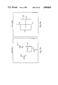
- FIG. 1 is a functional block diagram of the present invention.
- FIG. 2 is a diagram showing an extended application of the invention to three-dimensional scene constructing.
- FIG. 3 shows a camera model and corresponding coordinate system.
- FIG. 4 illustrates a successive application of horizontal and vertical rotation of the camera.
- FIG. 5 diagrams the effect of a focus of expansion location (FOE) for pure camera translation.
- FIG. 6 illustrates the concept of the FOE for discrete time steps during the motion of a vehicle having the camera.
- FIG. 7 shows the amount of expansion from the FOE for discrete time steps.
- FIGS. 8a and 8b display a displacement field caused by horizontal and vertical rotation and translation of the camera and a derotated displacement field, respectively.
- FIGS. 9a and 9b show an image plane and a rotation space, respectively.
- FIGS. 10a and 10b show mappings of a polygon from rotation space to an image plane and vice versa, respectively.
- FIGS. 11a-f illustrate a changing rotation polygon.
- FIG. 12 illustrates an intersection of displacement vectors with a vertical line which, if moved, changes the variance of intersection.
- FIG. 13 shows a displacement field used to evaluate various error functions.
- FIGS. 14a-d reveal the standard deviation of intersection at a vertical cross section at position x for different amounts of vertical rotation.
- FIGS. 15a-d reveal the standard deviation of intersection (square root) at a vertical cross section at position x for different amounts of vertical rotation with no horizontal rotation and with no pixel noise applied to the image locations.
- FIGS. 16a-d reveal the standard deviation of intersection (square root) at a vertical cross section at position x for different amounts of vertical rotation with no horizontal rotation and with ⁇ 1 pixels of noise applied to the image locations.
- FIGS. 17a-d reveal the standard deviation of intersection (square root) at a vertical cross section at position x for different amounts of vertical rotation with no horizontal rotation and with ⁇ 2 pixels of noise applied to the image locations.
- FIGS. 18a-d show the location of minimum intersection standard deviation under varying horizontal rotation with the horizontal location of the FOE marked xf.
- FIGS. 19a-d show the amount of minimum intersection standard deviation under varying horizontal rotation and with no noise added to the image locations.
- FIGS. 20a-d show the amount of minimum intersection deviation under varying horizontal rotation and with ⁇ 2 pixels noise added to the image locations.
- FIG. 21 illustrates intersecting displacement vectors with two vertical lines which lie on the same side of the FOE.
- FIGS. 22a-d show the correlation coefficient for the intersection of displacement vectors at two vertical lines under varying horizontal rotations with no noise added.
- FIGS. 23a-d show the correlation coefficient for the intersection of displacement vectors at two vertical lines under varying horizontal rotations and with ⁇ 2 pixels of noise added to the image locations.
- FIG. 24 illustrates displacement vectors and measurement of their error.
- FIG. 25 shows how to determine the optimum two-dimensional shift for a set of displacement vectors.
- FIG. 26 reveals how FOE locations are dismissed if the displacement field resulting from the application of the optimal shift results in a vector not pointing away from the FOE.
- FIGS. 27a-d illustrate the displacement field and minimum error at selected FOE locations.
- FIGS. 28a-e display the effects of increasing the average length of displacement vectors upon the shape of the error function.
- FIGS. 29a-e display the effects of increasing residual rotation in a horizontal direction upon the shape of the error function for relatively short vectors.
- FIGS. 30a-e display the effects of increasing residual rotation in a vertical direction upon the shape of the error function for relatively short vectors.
- FIGS. 31a-e show the effects of increasing residual rotation in horizontal and vertical directions upon the shape of the error function for relatively short vectors.
- FIGS. 31f-j indicate the amount of optimal linear shift obtained under the same conditions in FIGS. 31a-e.
- FIGS. 32a-e show the effects of the uniform noise applied to image point coordinates for a constant average vector length.
- FIGS. 33a and 33b reveal the different effects of uniform noise applied to image point coordinates for shorter and longer average vector lengths, respectively.
- FIG. 34 reveals a side view of a camera traveling parallel to a flat surface.
- FIGS. 35a-i show an original image sequence taken from a moving vehicle after edge detection and point detection with the selected points located at the lower-left corners of their marks.
- FIG. 35j-p show the original image sequence after edge detection and point selection.
- FIG. 36a-p illustrate the displacement vectors and estimates of vehicles motion for the image sequence shown in FIGS. 35a-p.
- FIG. 37 illustrates a specific hardware implementation of the embodiment of the invention.
- FIGS. 1 and 2 reveal the main portions of the present invention.
- FIG. 2 also expands on 3-D interpretations of 2-D images in items 118 and 120.
- Item 116 incorporates portions of items 122 and 124 of FIG. 1.
- significant features points, boundaries, corners, etc.
- points were selected and tracked between individual frames by item 114.
- Automatic techniques suitable for this task are in the related art.
- the vehicle's direction of translation i.e. the focus of expansion (FOE)
- FOE focus of expansion
- the effects of vehicle motion on the FOE computation is described below.
- the third step constructs an internal 3-D model of the scene. Also disclosed are the concepts and operation of the qualitative scene model 120. Experiments with the present invention on real imagery taken from a moving ALV are discussed below.
- System 110 contains the following three main components--token tracking 114, FOE seeker 124 and optimal derotation 122--in FIG. 1.
- the 2-D displacement vectors for selected image tokens are determined in the first stage (token tracking 114). Since those original displacement vectors are caused by some arbitrary and (at this point) unknown camera motion, including camera rotations, they do not yet exhibit the characteristic radial pattern of pure camera translation.
- the second component selects a set of candidate locations for the FOE and forms a connected image region of feasible FOE-locations plus the range of corresponding camera rotations, based on the results from the third component (optimal derotation 122).
- a particular FOE-location is feasible, if the corresponding error value (computed by the optimal derotation module 122) is below some dynamically adjusted threshold.
- the size of the final FOE-region reflects the amount of uncertainty contained in the visual information (large regions reflect high uncertainty).
- the third component determines the optimal 3-D camera rotations for a particular (hypothesized) FOE-location. This is accomplished by simulating the effects of reverse camera rotations upon the given set of displacement vectors. The camera is virtually rotated until the modified displacement field is closest to a radial expansion pattern with respect to the selected FOE-location. Module 122 returns the necessary amount of reverse rotation and the deviation from a radial displacement field (i.e., an error value).
- Component 123 comprising FOE seeker 124 and optimal derotation 122, represents the fuzzy FOE means which outputs the region of possible FOE locations.
- the first step of the present invention is to estimate the vehicle's motion relative to the stationary environment using visual information.
- Arbitrary movement of an object in 3-D space and thus the movement of the vehicle itself can be described as a combination of translation and rotation.
- knowledge about the composite vehicle motion is essential for control purposes, only translation can supply information about the spatial layout of the 3-D scene (motion stereo). This, however, requires the removal of all image effects results from vehicle rotation.
- FIG. 3 shows the camera-centered coordinate system 130, lens center 126, image plane 128, and angles ⁇ , ⁇ and ⁇ of rotation.
- the origin 0 of coordinate system 130 is located at lens center 126.
- Focal length f is the distance between lens center 126 and image plane 128.
- Each 3-D point (XYZ) may be mapped onto image location (X,Y).
- Angles ⁇ , ⁇ and ⁇ specify angles of camera rotation about the X,Y and Z axes, respectively.
- the camera is considered as being stationary and the environment as being moving as one single rigid object relative to the camera.
- the origin 0 of coordinate system 130 is located in the lens center 126 of the camera.
- the given task is to reconstruct the vehicle's or the camera's egomotion from visual information. It is therefore necessary to know the effects of different kings of vehicle or camera motion upon the camera image.
- the vehicle or camera undergoing rotation about the X-axis by an angle - ⁇ and the Y-axis by an angle - ⁇ moves each 3-D point X to point X' relative to the camera.
- the rotation mapping r.sub. ⁇ r.sub. ⁇ can also be separated into r.sub. ⁇ followed by r.sub. ⁇ .
- first step applying pure (horizontal) rotation around the Y-axis r.sub. ⁇ , point x 0 is moved to an intermediate image location x c .
- second step applying pure (vertical) rotation around the X-axis r.sub. ⁇ , takes point x c to the final image location x 1 . This can be expressed as ##EQU10##
- FIG. 4 reveals a successive application of horizontal and vertical rotation.
- Image point x 0 is to be moved to location x 1 by pure horizontal and vertical camera rotation.
- Horizontal rotation (about the Y-axis) is applied first, moving x 0 to x c , which is the intersection point of the two hyperbolic paths for horizontal and vertical rotation.
- x c is taken to x 1 .
- the two rotation angles ⁇ and ⁇ are found directly.
- FIG. 5 reveals the location of the FOE.
- points in the environment (A,B) move along 3-D vectors parallel to the vector pointing from lens center 126 to the FOE in camera plane 128 (FIG. 3). These vectors form parallel lines in space which have a common vanishing point (the FOE) in the perspective image.
- the straight line passing through the lens center of the camera and the FOE is also parallel to the 3-D displacement vectors. Therefore, the 3-D vector OF points in the direction of camera translation in space. Knowing the internal geometry of the camera (i.e., the focal length f), the direction of vehicle translation can be determined by locating the FOE in the image.
- the actual translation vector T applied to the camera is a multiple of the vector OF which supplies only the direction of camera translation but not its magnitude. Therefore,
- FIG. 6 illustrates the concept of FOE for discrete time steps.
- the motion of vehicle 132 between two points in time can be decomposed into a translation followed by a rotation.
- the image effects of pure translation (FOE a ) are observed in image I o .
- FIG. 6 shows the top view of vehicle 132 traveling along a curved path at two instances in time t 0 and t 1 .
- the position of the vehicle 132 in space is given by the position of a reference point on the vehicle P and the orientation of the vehicle is ⁇ .
- FIG. 6 also displays the adopted scheme of 3-D motion decomposition.
- the translation T is applied which shifts the vehicle's reference point (i.e., lens center 126 of the camera) from position P 0 to position P 1 without changing the vehicle's orientation ⁇ .
- the 3-D translation vector T intersects image plane 128 at FOE a .
- the vehicle is rotated b ⁇ to the new orientation ⁇ 1 .
- Translation T transforms image I 0 into image I' 1 , which again is transformed into I 1 by rotation ⁇ .
- FOE a is observed at the transition from image I 0 to image I' 1 , which is obtained by derotating image I 1 by - ⁇ .
- this scheme (FIG. 6) is used as a model for vehicle or camera motion.
- FIG. 7 shows the geometric relationships for the 2-D case. The amount of expansion from the FOE for discrete time steps is illustrated.
- FIG. 7 can be considered as a top view of the camera, i.e., a projection onto the X/Z-plane of the camera-centered coordinate system 130.
- the cross section of the image plane is shown as a straight line.
- the camera moves by a vector T in 3-D space, which passes through lens center 126 and the FOE in camera plane 128.
- the 3-D Z-axis is also the optical axis of the camera.
- the rate of expansion of image points from the FOE contains direct information about the distance of the corresponding 3-D points from the camera. Consequently, if the vehicle is moving along a straight line and the FOE has been located, the 3-D structure of the scene can be determined from the expansion pattern in the image.
- the distance Z of a 3-D point from the camera can only be obtained up tot he scale factor ⁇ Z, which is the distance that the vehicle advanced along the Z-axis during the elapsed time.
- the absolute range of any stationary point can be computed.
- the velocity of the vehicle can be obtained if the actual range of a point in the scene is known (e.g., from laser range data).
- any such technique requires that the FOE can be located in a small area, and the observed image points exhibit significant expansion away from the FOE. As shown below, imaging noise and camera distortion pose problems in the attempt to assure that both of the above requirements are met.
- the effects of camera translation T can be formulated as a mapping t of a set of image locations ⁇ x i ⁇ into another set of image locations ⁇ x' i ⁇ . Unlike in the case of pure camera rotation, this mapping not only depends upon the 3- D translation vector but also upon the actual 3-D location of each individual point observed. Therefore, in general, t is not simply a mapping of the image onto itself. However, one important property of t can be described exclusively in image plane 128, namely that each point must map onto a straight line passing through the original point and one unique location in the image (the FOE).
- FIG. 8a and 8b show a typical displacement field for a camera undergoing horizontal and vertical rotation as well as translation.
- the points x i ⁇ I are marked with small circles 138.
- Rectangle 134 marks the area of search for the FOE.
- the derotated displacement is illustrated in FIG. 8b with the FOE marked by circle 136.
- the vehicle's rotation and direction of translation in space can be computed from the information available in the image. This problem is addressed below.
- the 3-D motion M of the vehicle is modeled by a translation T followed by a rotation R.sub. ⁇ about the Y-axis and a rotation R.sub. ⁇ about the X-axis:
- the intermediate image I' 0 (26) is the result of the translation component of the vehicle's motion and has the property of being a radial mapping (23). Unlike the two images I 0 and I 1 , which are actually given, the image I' 0 is generally not observed, except when the camera rotation is zero. It serves as an intermediate result to be reached during the separation of translational and rotational motion components.
- AAV autonomous land vehicle
- the FOE may be obtained from rotation.
- the image motion is decomposed in two steps. First, the rotational components are estimated and their inverses are applied to the image, thus partially “derotating" the image. If the rotation estimate was accurate, the resulting displacement field after derotation would diverge from a single image location (the FOE). The second step verifies that the displacement field is actually radial and determines the location of the FOE. For this purpose, two problems have to be solved: (1) how to estimate the rotational motion components without knowing the exact location of the FOE, and (2) how to measure the "goodness of derotation" and locate the FOE.
- Each vector in the displacement field is the sum of vector components caused by camera rotation and camera translation. Since the displacement caused by translation depends on the depth of the corresponding points in 3-D space (equation 18), points located at a large distance from the camera are not significantly affected by camera translation. Therefore, one way of estimating vehicle rotation is to compute ⁇ and ⁇ from displacement vectors which are known to belong to points at far distance. Under the assumption that those displacement vectors are only caused by rotation, equations 14 and 15 can be applied to find the two angles. In some situations, distant points are selected easily. For example, points on the horizon are often located at a sufficient distance from the vehicle. Image points close to the axis of translation would be preferred because they expand from the FOE slower than other points at the same depth.
- FIG. 9a shows an image plane which illustrates this situation.
- the FOE of the previous frame was located at the center of square 140 which outlines the region of search for the current FOE, thus the FOE in the given frame must be inside square 140.
- the main idea of this technique is to determine the possible range of camera rotations which would be consistent with the FOE lying inside marked region 140. Since the camera rotates about two axes, the resulting range of rotations can be described as a region in a 2-D space.
- FIG. 9b shows this rotation space with the two axes ⁇ and ⁇ corresponding to the amount of camera rotation around the Y-axis and the X-axis, respectively.
- the initial rotation estimate is a range of ⁇ 10° in both directions which is indicated by a square 142 in rotation space of FIG. 9b.
- the range of possible rotations is described by a closed, convex polygon in rotation space.
- a particular rotation ( ⁇ ', ⁇ ') is possible if its application to every displacement vector (i.e., to its endpoint) yields a new vector which lies on a straight line passing through the maximal FOE-region.
- the region of possible rotations is successively constrained by applying the following steps for every displacement vector (FIG. 10a and 10b).
- Polygon 148 is similar to the rotation polygon 144 but distorted by the nonlinear rotation mapping as shown in FIG. 10a.
- rotation polygon 158 is empty (number of vertices is zero), then stop. No camera rotation is possible that would make all displacement vectors intersect the given FOE-region. Repeat the process using a larger FOE-region.
- FIGS. 11a, 11b and 11c show the changing shape of the rotation polygon during the application of this process to the three displacement vectors in FIG. 8.
- FIG. 11a shows rotation polygon after examining displacement vector P1 ⁇ P1'. Any camera rotation inside the polygon would move the endpoint of the displacement vector (P1') into the open triangle formed by targets 164 and 166 through P1 to the maximal FOE-region given by square 68 in the image plane.
- the actual mapping of the rotation polygon into the image plane is shown with a dotted outline.
- FIG. 11b reveals the rotation polygon 170 after examining displacement vectors P1 ⁇ P1' and P2 ⁇ P2'.
- FIG. 11(c) shows the final rotation polygon after examining the three displacement vectors P1 ⁇ P1', P2 ⁇ P2'and P3 ⁇ P3'.
- the amount of camera rotation can be constrained to a range of below 1° in both directions. Rotation can be estimated more accurately when the displacement vectors are short, i.e., when the amount of camera translation is small. This is in contrast to estimating camera translation which is easier with long displacement vectors.
- the situation when the rotation polygon becomes empty requires some additional considerations. As mentioned earlier, in such a case no camera rotation is possible that would make all displacement vectors pass through the given FOE-region. This could indicate one of the two alternatives.
- This algorithm searches for the smallest feasible FOE-region by systematically discarding sub regions from further consideration. For the case that the shape of the original region is a square, subregions can be obtained by splitting the region into four subsquares of equal size.
- the simple version shown here performs a depth-first search down to the smallest subregion (limited by the parameter "min-size"), which is neither the most elegant nor the most efficient approach.
- the algorithm can be significantly improved by applying a more sophisticated strategy, for example, by trying to discard subregions around the perimeter first before examining the interior of a region. Two major problems were encountered with the latter method. First, the algorithm is computationally expensive since the process of computing feasible rotations must be repeated for every subregion. Second, a small region is more likely to be discarded than a larger one. However, when the size of the region becomes too small, errors induced by noise, distortion or point-tracking may prohibit displacement vectors from passing though a region which actually contains the FOE.
- Locating the FOE in a partially derotated image may be attempted. After applying a particular derotation mapping to the displacement field, the question is how close the new displacement field is to a radial mapping, where all vectors diverge from one image location. If the displacement field is really radial, then the image is completely derotated and only the components due to camera translation remain. Two different methods for measuring this property are noted. One method used the variance of intersection at imaginary horizontal and vertical lines. The second method computes the linear correlation coefficient to measure how "radial" the displacement field is. The variance of intersection in related art suggests to estimate the disturbance of the displacement field by computing the variance of intersections of one displacement vector with all other vectors.
- FIG. 12 shows 5 displacement vectors P 1 ⁇ P' . . . P 5 ' intersecting a vertical line at x at y 1 . . . Y 5 . Moving the vertical line from x towards x 0 will bring the points of intersection closer together and will thus result in a smaller variance of intersection.
- the point of intersection of a displacement vector P i ⁇ P i ' with a vertical line at x is given by ##EQU19##
- the variance of intersection of all displacement vectors with the vertical line at position x is ##EQU20##
- the first derivative of (29) with respect to x is set to zero.
- the location x 0 of minimum intersection variance is then obtained.
- the position of a horizontal cross section with minimal intersection variance can be obtained.
- the square root of the variance of intersection (standard deviation) at a vertical line was evaluated on the synthetic displacement field shown in FIG. 13.
- the actual FOE is located in the center of the image.
- Square 174 around the center ( ⁇ 100 pixels in both directions) marks the region over which the error functions are evaluated.
- FIGS. 14a, b, c and d show the distribution of the intersection standard deviation for increasing residual rotations in vertical direction in the absence of noise.
- the horizontal rotation is 1° in all cases represented by these Figures. Locations of displacement vectors are presented by real numbers (not rounded to integer values).
- no residual rotation exists i.e., the displacement field is perfectly radial.
- the value of the horizontal position of the cross section varies ⁇ 100 pixels around the actual FOE.
- the residual vertical rotation is increased from 0.2° to 1.0°.
- the bold vertical bar marks the horizonal position of minimum standard deviation
- the thin bar marks the location of the FOE (X f ). It can be seen that the amount of minimum standard deviation rises with increasing disturbance by rotation, but that the location of minimum standard deviation does not necessarily move away from the FOE.
- FIGS. 15-17 show the same function under the influence of noise.
- noise was applied except that by merely rounding the locations of displacement vectors to their nearest integer values.
- These Figures show standard deviation of intersection (square root) at a vertical cross section at position x for different amounts of vertical rotation with no horizontal rotation.
- Uniform noise of ⁇ 1 pixels was added to the image locations in FIGS. 16a-d.
- uniform noise of ⁇ 2 pixels was applied to the image locations. It can be seen that the effects of noise are similar to the effects caused by residual rotation components.
- the purpose of this error function is to determine where the FOE is located, and how "radial" the current displacement field is.
- FIG. 18a-d plot the location of minimum intersection standard deviation under varying horizontal rotation. The vertical rotation is kept fixed for each plot. Horizontal camera rotations from -1° to +1° are shown on the abscissa (rot). The ordinate (x0) gives the location of minimum standard deviation in the range of ⁇ 100 pixels around the FOE (marked xf). The location of minimum standard deviation depends strongly on the amount of horizontal rotation.
- a problem is that the location of minimum standard deviation is not necessarily closer to the FOE when the amount of rotation is less.
- the function is only well behaved in a narrow range around zero rotation, which means that the estimate of the camera rotation must be very accurate to successfully locate the FOE.
- the second purpose of this error function is to measure how "radial" the displacement field is after partial derotation. This should be possible by computing the amount of minimum intersection standard deviation. Intuitively, a smaller amount of minimum intersection standard deviation should indicate that the displacement field is less disturbed by rotation.
- FIGS. 19a-d and 20a-d show that this is generally true by showing the amount of minimum intersection standard deviation under varying horizontal rotation. For the noise-free case in FIG.
- FIGS. 19a-d show the same function in the presence of ⁇ 2 pixels of uniform noise added to image locations.
- the second method, utilizing linear correlation, of measuring how close a displacement field is to a radial pattern again uses the points y 11 -y 15 and y 21 -y 25 of intersection at vertical (or horizontal) lines x 1 and x 2 as illustrated in FIG. 21.
- the displacement vectors P 1 ⁇ P' 1 through P 5 ⁇ P' 5 are intersected by two vertical lines X 1 and X 2 , both of which lie on the same side of the FOE that is within area 176. Since the location of the FOE is not known, the two lines X 1 and X 2 are simply located at a sufficient distance from any possible FOE-location.
- FIGS. 22a-d and 23a-d show plots for the correlation coefficient for intersection of displacement vectors at two vertical lines under varying horizontal rotations, under the same conditions as in FIGS. 19a-d and 20a-d.
- No noise was applied for FIG. 22a-d.
- FIGS. 23a-d a uniform noise of ⁇ 2 pixels was added to the image locations.
- the optimal coefficient is +1.0 (horizontal axis) in FIGS. 22a-d.
- the shapes of the curves of FIGS. 22a-d and 23a-d are similar, respectively, to FIGS. 19a-d and 20a-d for the minimum standard deviations shown above earlier, with peaks at the same locations.
- An initial guess for the FOE-location is obtained from knowledge about the orientation of the camera with respect to the vehicle.
- the FOE-location computed from the previous pair can be used as a starting point.
- the problem is to compute the rotation mappings r.sub. ⁇ -1 and r.sub. ⁇ -1 which, when applied to the image I 1 , will result in an optimal radial mapping with respect to I 0 and x f .
- the perpendicular distances between points in the second image (x' i ) and the "ideal" displacement vectors is measured.
- the "ideal" displacement vectors line on straight lines passing through the the FOE x f and the points in the first image x i (see FIG. 24) which illustrates measuring the perpendicular distance d i between lines from x f through points x i in the second image.
- the sum of the squared perpendicular distances d i is the final error measure. For each set of corresponding image points (x i ⁇ I, x' i ⁇ I'), the error measure is defined as ##EQU22##
- FIG. 26 shows a field of 5 displacement vectors.
- the optimal shift s opt for the given x f is shown as a vector in the lower right-hand corner.
- the final algorithm for determining the direction of heading as well as horizontal and vertical camera rotations is the "find-FOE algorithm" which consists the steps: (1) Guess an initial FOE x f 0 , for example the FOE-location obtained from the previous pair of frames; (2) Starting from x f 0 , search for a location x f opt where E min (x f opt ) is a minimum. A technique of steepest descent is used, where the search proceeds in the direction of least error; and (3) Determine a region around x f opt in which the error is below some threshold.
- the search for this FOE-area is conducted at FOE-locations lying on a grid of fixed width. In the examples shown, the grid spacing is 10 pixels on both x- and y-directions.
- the error function E(x f ) is computed in time proportional to the number of displacement vectors N.
- the final size of the FOE-area depends on the local shape of the error function and can be constrained not to exceed a certain maximum M. Therefore, the time complexity is O(MN).
- FIGS. 27a-d shows the distribution of the normalized error E n (x f ) for a sparse and relatively short displacement field containing 7 vectors. Residual rotation components of ⁇ 2° in horizontal and vertical direction are present in FIGS. 27b-d to visualize their effects upon the image. This displacement field was used with different average vector lengths (indicated as length-factor) for the other experiments on synthetic data.
- the displacement vector through the guiding point is marked with a heavy line.
- the choice of this point is not critical, but it should be located at a considerable distance from the FOE to reduce the effects of noise upon the direction of the vector x f x g .
- FIGS. 27a-d which show displacement field and minimum error at selected FOE-locations, the error function is sampled in a grid with a width of 10 pixels over an area of 200 by 200 pixels around the actual FOE, which is marked by small square 178.
- the amount of normalized error is (equation 41) indicated by the size of the circle 180.
- Heavy circles 180 indicate error values which are above a certain threshold.
- FIG. 27a represents no residual rotation
- FIG. 27b represents 2.0° of horizontal camera rotation (to the left)
- FIG. 27c represents 2.0° of vertical rotation (upwards)
- FIG. 27d represents -2.0° vertical rotation (downwards).
- FIGS. 28 to 33 show the effects of various conditions upon the behavior of this error function in the same 200 by 200 pixel square round the actual FOE as in FIGS. 27a-d.
- FIGS. 28a-e show how the shape of the error function depends upon the average length (with length factors varying from 1 to 15) of the displacement vectors in the absence of any residual rotation or noise (except digitization noise). The minimum of the error function becomes more distinct with increasing amounts of displacement.
- FIGS. 29a-e show the effect of increasing residual rotation in horizontal direction upon the shape of the error function for relatively short vectors (length factor of 2.0) in absence of noise.
- FIGS. 30a-e show the effect of residual rotation in vertical direction upon the shape of the error function for short vectors (length factor of 2.0) in absence of noise.
- the displacement field used is extremely nonsymmetric along the Y-axis of the image plane. This is motivated by the fact that in real ALV images, long displacement vectors are most likely to be found from points on the ground, which are located in the lower portion of the image. Therefore, positive and negative vertical rotations have been applied in FIGS. 30a-e.
- FIGS. 31a-j residual rotations in both horizontal and vertical direction, respectively, are present, for short vectors with a length factor of 2.0.
- the error function is quite robust against rotational components in the image.
- FIGS. 31f-j show the amounts of optimal linear shift s opt under the same conditions.
- the result in FIG. 31e shows the effect of large combined rotation of 4.0°/4.0° in both directions.
- the minimum of the error function is considerably off the actual location of the FOE because of the error induced by using a linear shift to approximate the nonlinear derotation mapping. In such a case, it would be necessary to actually derotate the displacement field by the amount of rotation equivalent to s opt found at the minimum of this error function and repeat the process with the derotated displacement.
- FIGS. 32a-e The effects of various amounts of uniform noise applied to image point coordinates for a constant average vector length of 5.0, are shown in FIGS. 32a-e.
- a random amount (with uniform distribution) of displacement was added to the original (continuous) image location and then rounded to integer pixel coordinates.
- Random displacement was applied in ranges from ⁇ 0.5 to ⁇ 4.0 pixels in both horizontal and vertical direction.
- the shape of the error function becomes flat around the local minimum of the FOE with increasing levels of the noise.
- the displacement field contains only 7 vectors. What is observed here is that the absolute minimum error increases with the amount of noise.
- FIGS. 32a-e thus serve as an indicator for the amount of noise present in the image and the reliability of the final result.
- FIGS. 33a and 33b show the error functions for two displacement fields with different average vector lengths (length factor 2.0 and 5.0, respectively).
- length-factor 2.0 the shape of the error function changes dramatically under the same amount of noise (compare FIG. 31a).
- a search for the minimum error i.e., local minimum ) inevitably converge towards an area 182 indicated by the small arrow, far off the actual FOE.
- the minimum of the error function coincides with the actual location of the FOE 178.
- velocity over ground may be computed.
- the FOE has been computed following the steps outlined above, the direction of vehicle translation and the amount of rotation are known.
- the 3-D layout of the scene can be obtained up to a common scale factor (equation 20).
- this scale factor and, consequently, the velocity of the vehicle can be determined if the 3-D position of one point in space is known. Furthermore, it is easy to show that it is sufficient to know only one coordinate value of a point in space to reconstruct its position in space from its location in the image.
- FIG. 34 shows a side view of camera 184 traveling parallel to flat surface 186.
- Camera 184 advances in direction Z, such that a 3-D point on ground surface 186 moves relative to camera 184 from Z 0 to Z 1 .
- Depression angle ⁇ can be determined from the location of FOE 188 in image 128. Height of camera 184 above ground surface 186 is given.
- a coordinate system 130 which has its origin O in the lens center 126 of the camera 184.
- the Z-axis of coordinate system 130 passes through FOE 188 in the image plane 128 and aims in the direction of translation.
- the original camera-centered coordinate system (X Y Z) 130 is transformed into the new frame (X' Y' Z') merely by applying horizontal and vertical rotation until the Z-axis lines-up with FOE 188.
- the horizontal and vertical orientation in terms of "pan” and "tilt” are obtained by "rotating" FOE 188 (x f y f ) into the center of image 128 (OO) using equations 14 and 15 in the following: ##EQU28##
- the two angles ⁇ f and ⁇ f represent the orientation of camera 184 in 3-D with respect to the new coordinate system (X' Y' Z'). This allows determination of the 3-D orientation of the projecting rays passing through image points y 0 and y 1 by use of the inverse perspective transformation.
- A3-D point X in the environment whose image x (xy) is given, lies on a ##EQU29##
- the Y-coordinate is -h which is the height of camera 184 above ground 186. Therefore, the value of ⁇ s for a point on the road surface (x s y s ) can be estimated as ##EQU30## and its 3-D distance is found by inserting ⁇ s into equation 41 as ##EQU31##
- results of the FOE-algorithm and computation of the vehicle's velocity over ground are shown on a real image sequence taken from the moving ALV.
- the original sequence was provided on standard video tape with a frame-rate of 30 per second.
- images were taken in 0.5 second intervals, i.e., at a frame rate of 2 per second in order to reduce the amount of storage and computation.
- the images were digitized to a spatial resolution of 512 ⁇ 512, using only the Y-component (luminance) of the original color signal.
- FIGS. 35a-i show the edge image of frames 182-190 of an actual test, with points 1-57 being tracked and labeled with ascending numbers.
- FIGS. 35a-i show the original image sequence taken from the moving ALV after edge detection and point detection. Selected points 1-57 are located at the lower-left corners of their marks.
- FIGS. 35j-p (frames 191-197), which include additional points 58-78, show the original image sequence taken after edge detection and point selection.
- An adaptive windowing technique was developed as an extension of relaxation labeling disparity analysis for the selection and matching of tracked points. The actual image location of each point is the lower left corner of the corresponding mark.
- the resulting data structure consists of a list of point observations for each image (time), e.g., time t o : ((P 1 t 0 x 1 y 1 ) (P 2 t 0 x 2 y 2 ) (P 3 t 0 x 3 y 3 ) . . . ) time t 1 : ((P 1 t 1 x 1 y 1 ) (P 2 t 1 x 2 y 2 ) (P 3 t 1 x 3 y 3 ) . . . )
- Points are given a unique label when they are encountered for the first time. After the tracking of a point has started, its label remains unchanged until this point is no longer tracked. When no correspondence is found in the subsequent frame for a point being tracked, either because of occlusion, or the feature left the field of view, or because it could not be identified, tracking of this point is discontinued. Should the same point reappear again, it is treated as a new item and given a new label. Approximately 25 points per image have been selected in the sequence shown in FIGS. 35a-i. In the search for the focus of expansion, the optical FOE-location from the previous pair of frames is taken as the initial guess.
- the location of the FOE is guessed from the known camera setup relative to the vehicle.
- the points which are tracked on the two cars (24 and 33) are assumed to be known as moving and are not used as reference points to compute the FOE, vehicle rotation, and velocity. This information is eventually supplied by the reasoning processes in conjunction with the qualitative scene model (FIG. 2).
- FIGS. 36a-p illustrative the displacement vectors and estimates of vehicle motion for the image sequence shown in FIGS. 35a-p.
- shaded area 190 marks the possible FOE locations and circle 178 inside of area 190 is the FOE with the lowest error value.
- the FOE-ratio measures the flatness of the error function inside area 190.
- FIGS. 36a-p show the results of computing the vehicle's motion for the same sequence as in the previous Figure.
- Each frame t displays the motion estimates for the period between t and the previous frame t-1. Therefore, no estimate is available at the first frame (182).
- the FOE-algorithm first searches for the image location, which is not prohibited and where the error function (equation 35) has a minimum.
- the optimal horizontal and vertical shift resulting at this FOE-location is used to estimate the vehicle's rotations around the X- and Y-axis. This point, which is the initial guess for the subsequent frame, is marked as a small circle inside the shaded area.
- the equivalent rotation components are shown graphically on a ⁇ 1° scale. They are relatively small throughout the sequence such that it was never necessary to apply intermediate derotation and iteration of the FOE-search. Along with the original displacement vectors (solid lines), the vectors obtained after derotation are shown with dashed lines.
- the location with minimum error After the location with minimum error has been found, it is used as the seed for growing a region of potential FOE-locations.
- the growth of the region is limited by two restrictions: (1) The ratio of maximum to minimum error inside the region is limited, i.e.,
- FIG. 37 illustrates hardware embodiment 200 of the present invention.
- Camera 202 may be a Hitachi television camera having a 48° vertical field of view and a 50° horizontal field of view. Camera 202 may be set at a depression angle of 16.3° below the horion.
- Image sequence 204 acquired by camera 202 are transmitted to tracking means 206 comprising an I 2 S processor 208 and a VAX 11/750 computer 210. Tracking means 206 tracks tokens between frames of image sequences 204. The output of means 206 goes to means 212 for matching of tokens and corresponding images.
- a VAX-Symbolics bidirectional network protocol means 214 is connected between means 212 and means 216 which includes Symbolics 3670 computer 218, though it is possible to use one computer thereby eliminating means 214.
- Computer 218 provides processing for obtaining fuzzy focus of expansion and rotations/translation estimates of motion.
- the language environment used with computer 218 is Common LISP.
Abstract
Determining the self-motion in space of an imaging device (e.g., a television camera) by analyzing image sequences obtained through the device. Three-dimensional self-motion is expressed as a combination of rotations about the horizontal and vertical camera axes and the direction of camera translation. The invention computes the rotational and translational components of the camera self-motion exclusively from visual information. Robust performance is achieved by determining the direction of heading (i.e., the focus of expansion) as a connected region instead of a single location on the image plane. The method can be used to determine when the direction of heading is outside the current field of view and when there is zero or very small camera translation.
Description
The present invention pertains to imaging and particularly to three-dimensional interpretation of two-dimensional image sequences. More particularly, the invention pertains to determination of three-dimensional self-motion of moving imaging devices.
Visual information is an indispensable clue for the successful operation of an autonomous land vehicle. Even with the use of sophisticated inertial navigation systems, the accumulation of position error requires periodic corrections. Operation in unknown environments or mission tasks involving search, rescue, or manipulation critically depend upon visual feedback.
Assessment of scene dynamics becomes vital when moving objects may be encountered, e.g., when the autonomous land vehicle follows a convoy, approaches other vehicles, or has to detect moving threats. For the given case of a moving camera, such as one mounted on the autonomous land vehicle, image motion can supply important information about the spatial layout of the environment ("motion stereo") and the actual movements of the land vehicle.
Previous work in motion analysis has mainly concentrated on numerical approaches for the recovery of three-dimensional (3-D) motion and scene structure from two-dimensional (2-D) image sequences. The most common approach is to estimate 3-D structure and motion in one computational step by solving a system of linear or non-linear equations. This technique is characterized by several severe limitations. First, it is known for its notorious noise-sensitivity. To overcome this problem, some researchers have extended this technique to cover multiple frames. Secondly, it is designed to analyze the relative motion and 3-D structure of a single rigid object. To estimate the egomotion of an autonomous land vehicle (ALV), having the imaging device or camera, and the accompanying scene structure, the environment would have to be treated as a large rigid object. However, rigidness of the environment cannot be guaranteed due to the possible presence of moving objects in the scene. The consequence of accidentally including a moving 3-D point into the system of equations, representing the imaged environment, in the best case, would be a solution (in terms of motion and structure) exhibiting a large residual error, indicating some non-rigid behavior. The point in motion, however, could not be immediately identified from this solution alone. In the worst case (for some forms of motion), the system may converge towards a rigid solution (with small error) in spite of the actual movement in the point set. This again shows another (third) limitation: there is no suitable means of expressing the ambiguity and uncertainty inherent to dynamic scene analysis. The invention, that solves the aforementioned problems, is novel in two important aspects. The scene structure is not treated as a mere by-product of the motion computation but as a valuable means to overcome some of the ambiguities of dynamic scene analysis. The key idea is to use the description of the scene's 3-D structure as a link between motion analysis and other processes that deal with spatial perception, such as shape-from-occlusion, stereo, spatial reasoning, etc. A 3-D intepretation of a moving scene can only be correct if it is acceptable by all the processes involved.
Secondly, numeral techniques are largely replaced by a qualitative strategy of reasoning and modeling. Basically, instead of having a system of equations approaching a single rigid (but possibly incorrect) numerical solution, multiple qualitative interpretations of the scene are maintained. All the presently existing interpretations are kept consistent with the observations made in the past. The main advantage of this approach of the present invention is that a new interpretation can be supplied immediately when the currently favored interpretation turns out to be unplausible.
The problem of determining the motion parameters of a moving camera relative to its environment from a sequence of images is important for applications for computer vision in mobile robots. Short-term control, such as steering and braking, navigation, and obstacle detection/avoidance are all tasks that can effectively utilize this information.
The present invention deals with the computation of sensor platform motion from a set of displacement vectors obtained from consecutive pairs of images. It is directed for application to autonomous robots and land vehicles. The effects of camera rotation and translation upon the observed image are overcome. The new concept of "fuzzy" focus of expansion (FOE), which marks the direction of vehicle heading (and provides sensor rotation), is exploited. It is shown that a robust performance for FOE location can be achieved by computing a 2-D region of possible FOE-locations (termed "Fuzzy FOE") instead of looking for a single-point FOE. The shape of this FOE is an explicit indicator of the accuracy of the result. Given the fuzzy FOE, a number of very effective inferences about the 3-D scene structure and motion are possible and the fuzzy FOE can be employed as a practical tool in dynamic scene analysis. The results are realized in real motion sequences.
The problem of understanding scene dynamics is to find consistent and plausible 3-D interpretations for any change observed in the 2-D image sequence. Due to the motion of the autonomous land vehicle (ALV), containing the scene sensing device, stationary objects in the scene generally do not appear stationary in the image, whereas moving objects are not necessarily seen in motion. The three main tasks of the present approach for target motion detection and tracking are: (1) to estimate the vehicle's motion; (2) to derive the 3-D structure of the stationary environment; and (b 3) to detect and classify the motion of individual targets in the scene. These three tasks are interdependent. The direction of heading (i.e., translation) and rotation of the vehicle are estimated with respect to stationary locations in the scene. The focus of expansion (FOE) is not determined as a particular image location, but as a region of possible FOE-locations called the fuzzy FOE. We present a qualitative strategy of reasoning and modeling for the perception of 3-D space from motion information. Instead of refining a single quantitative description of the observed environment over time, multiple qualitative interpretations are maintained simultaneously. This offers superior robustness and flexibility over traditional numerical techniques which are often ill-conditioned and noise-sensitive. A rule-based implementation of this approach is discussed results on real ALV imagery are presented.
The system of the present invention tracks stationary parts of the visual environment in the image plane, using corner points, contour segments, region boundaries and other two-dimensional tokens as references. This results in a set of 2-D displacement vectors for the selected tokens for each consecutive pair of camera images. The self-motion of the camera is modeled as two separate rotations about horizontal and the vertical axes passing through the lens center and a translation in 3-D space. If the camera performs pure translation along a straight line in 3-D space, then (theoretically) all the displacement vectors extend through one particular location in the image plane, called the focus of expansion (FOE) under forward translation or focus of contraction (FOC) under backward translation. The 3-D vector passing through the lens center and the FOE (on the image plane) corresponds to the direction of camera translation in 3-D space.
The invention can provide the directions of instantaneous heading of the vehicle (FOE) within 1° and self motions of moving imaging devices can be accurately obtained. This includes rotations of ±5° or larger in horizontal and vertical directions. To cope with the problems of noise and errors in the displacement field, a region of possible FOE-locations (i.e., the fuzzy FOE) is determined instead of a single FOE.
In practice, however, imaging noise, spatial discretization errors, etc., make it impractical to determine the FOE as an infinitesimal image location. Consequently, a central strategy of our method is to compute a region of possible FOE-locations (instead of a single position) which produces more robust and reliable results than previous approaches.
FIG. 1 is a functional block diagram of the present invention.
FIG. 2 is a diagram showing an extended application of the invention to three-dimensional scene constructing.
FIG. 3 shows a camera model and corresponding coordinate system.
FIG. 4 illustrates a successive application of horizontal and vertical rotation of the camera.
FIG. 5 diagrams the effect of a focus of expansion location (FOE) for pure camera translation.
FIG. 6 illustrates the concept of the FOE for discrete time steps during the motion of a vehicle having the camera.
FIG. 7 shows the amount of expansion from the FOE for discrete time steps.
FIGS. 8a and 8b display a displacement field caused by horizontal and vertical rotation and translation of the camera and a derotated displacement field, respectively.
FIGS. 9a and 9b show an image plane and a rotation space, respectively.
FIGS. 10a and 10b show mappings of a polygon from rotation space to an image plane and vice versa, respectively.
FIGS. 11a-f illustrate a changing rotation polygon.
FIG. 12 illustrates an intersection of displacement vectors with a vertical line which, if moved, changes the variance of intersection.
FIG. 13 shows a displacement field used to evaluate various error functions.
FIGS. 14a-d reveal the standard deviation of intersection at a vertical cross section at position x for different amounts of vertical rotation.
FIGS. 15a-d reveal the standard deviation of intersection (square root) at a vertical cross section at position x for different amounts of vertical rotation with no horizontal rotation and with no pixel noise applied to the image locations.
FIGS. 16a-d reveal the standard deviation of intersection (square root) at a vertical cross section at position x for different amounts of vertical rotation with no horizontal rotation and with ±1 pixels of noise applied to the image locations.
FIGS. 17a-d reveal the standard deviation of intersection (square root) at a vertical cross section at position x for different amounts of vertical rotation with no horizontal rotation and with ±2 pixels of noise applied to the image locations.
FIGS. 18a-d show the location of minimum intersection standard deviation under varying horizontal rotation with the horizontal location of the FOE marked xf.
FIGS. 19a-d show the amount of minimum intersection standard deviation under varying horizontal rotation and with no noise added to the image locations.
FIGS. 20a-d show the amount of minimum intersection deviation under varying horizontal rotation and with ±2 pixels noise added to the image locations.
FIG. 21 illustrates intersecting displacement vectors with two vertical lines which lie on the same side of the FOE.
FIGS. 22a-d show the correlation coefficient for the intersection of displacement vectors at two vertical lines under varying horizontal rotations with no noise added.
FIGS. 23a-d show the correlation coefficient for the intersection of displacement vectors at two vertical lines under varying horizontal rotations and with ±2 pixels of noise added to the image locations.
FIG. 24 illustrates displacement vectors and measurement of their error.
FIG. 25 shows how to determine the optimum two-dimensional shift for a set of displacement vectors.
FIG. 26 reveals how FOE locations are dismissed if the displacement field resulting from the application of the optimal shift results in a vector not pointing away from the FOE.
FIGS. 27a-d illustrate the displacement field and minimum error at selected FOE locations.
FIGS. 28a-e display the effects of increasing the average length of displacement vectors upon the shape of the error function.
FIGS. 29a-e display the effects of increasing residual rotation in a horizontal direction upon the shape of the error function for relatively short vectors.
FIGS. 30a-e display the effects of increasing residual rotation in a vertical direction upon the shape of the error function for relatively short vectors.
FIGS. 31a-e show the effects of increasing residual rotation in horizontal and vertical directions upon the shape of the error function for relatively short vectors.
FIGS. 31f-j indicate the amount of optimal linear shift obtained under the same conditions in FIGS. 31a-e.
FIGS. 32a-e show the effects of the uniform noise applied to image point coordinates for a constant average vector length.
FIGS. 33a and 33b reveal the different effects of uniform noise applied to image point coordinates for shorter and longer average vector lengths, respectively.
FIG. 34 reveals a side view of a camera traveling parallel to a flat surface.
FIGS. 35a-i show an original image sequence taken from a moving vehicle after edge detection and point detection with the selected points located at the lower-left corners of their marks.
FIG. 35j-p show the original image sequence after edge detection and point selection.
FIG. 36a-p illustrate the displacement vectors and estimates of vehicles motion for the image sequence shown in FIGS. 35a-p.
FIG. 37 illustrates a specific hardware implementation of the embodiment of the invention.
FIGS. 1 and 2 reveal the main portions of the present invention. FIG. 2 also expands on 3-D interpretations of 2-D images in items 118 and 120. Item 116 incorporates portions of items 122 and 124 of FIG. 1. First, significant features (points, boundaries, corners, etc.) are extracted by feature extraction and tracking 114 from the image data 112 and the 2-D displacement vectors are computed for this set of features. For the examples shown here, points were selected and tracked between individual frames by item 114. Automatic techniques suitable for this task are in the related art. In the second step, the vehicle's direction of translation, i.e. the focus of expansion (FOE), and the amount of rotation in space are determined. The effects of vehicle motion on the FOE computation is described below. Nearly all the necessary numerical computation is perforated in the FOE computation stage, which also is described below. The third step (at 2-D change analysis 118) constructs an internal 3-D model of the scene. Also disclosed are the concepts and operation of the qualitative scene model 120. Experiments with the present invention on real imagery taken from a moving ALV are discussed below.
The second component (FOE seeker 124) selects a set of candidate locations for the FOE and forms a connected image region of feasible FOE-locations plus the range of corresponding camera rotations, based on the results from the third component (optimal derotation 122). A particular FOE-location is feasible, if the corresponding error value (computed by the optimal derotation module 122) is below some dynamically adjusted threshold. The size of the final FOE-region reflects the amount of uncertainty contained in the visual information (large regions reflect high uncertainty).
The third component (optimal derotation 122) determines the optimal 3-D camera rotations for a particular (hypothesized) FOE-location. This is accomplished by simulating the effects of reverse camera rotations upon the given set of displacement vectors. The camera is virtually rotated until the modified displacement field is closest to a radial expansion pattern with respect to the selected FOE-location. Module 122 returns the necessary amount of reverse rotation and the deviation from a radial displacement field (i.e., an error value).
The first step of the present invention is to estimate the vehicle's motion relative to the stationary environment using visual information. Arbitrary movement of an object in 3-D space and thus the movement of the vehicle itself can be described as a combination of translation and rotation. While knowledge about the composite vehicle motion is essential for control purposes, only translation can supply information about the spatial layout of the 3-D scene (motion stereo). This, however, requires the removal of all image effects results from vehicle rotation. For this purpose, we discuss the changes upon the image that are caused by individual application of the "pure" motion components.
It is well-known that any rigid motion of an object in space between two points in time can be decomposed into a combination of translation and rotation. While many researchers have used a velocity-based formulation of the problem, the following treatment views motion in discrete time steps.
The viewing geometry involves a world coordinate system, (XYZ) as illustrated in FIG. 3. FIG. 3 shows the camera-centered coordinate system 130, lens center 126, image plane 128, and angles φ, θ and ψ of rotation. The origin 0 of coordinate system 130 is located at lens center 126. Focal length f is the distance between lens center 126 and image plane 128. Each 3-D point (XYZ) may be mapped onto image location (X,Y). Angles φ, θ and ψ specify angles of camera rotation about the X,Y and Z axes, respectively. Given the world coordinate system, a translation T=(U V W)T applied to a point in 3-D X=(X Y Z)T is accomplished through vector addition: ##EQU1## A 3-D rotation R about an arbitrary axis through the origin of coordinate system 130 can be described by successive rotations about its three axes: ##EQU2##
A general rigid motion in space consisting of translation and rotation is described by the transformation
M:X→X'=R.sub.φ R.sub.θ R.sub.ψ (T+X) (4)
Its six degrees of freedom are U, V, W, φ, θ, ψ.
This decomposition is not unique because the translation could be as well applied after the rotation. Also, since the multiplication of the rotation matrices is not commutative, a different order of rotations would result in different amounts of rotation for each axis. For a fixed order of application, however, this motion decomposition is unique.
To model the movements of the vehicle, the camera is considered as being stationary and the environment as being moving as one single rigid object relative to the camera. The origin 0 of coordinate system 130 is located in the lens center 126 of the camera.
The given task is to reconstruct the vehicle's or the camera's egomotion from visual information. It is therefore necessary to know the effects of different kings of vehicle or camera motion upon the camera image. Under perspective imaging, a point in space X=(X Y Z)T is projected onto a location on the image plane X=(X Y)T such that ##EQU3## where f is the focal length of the camera (see FIG. 3).
The effects of pure camera rotation are accounted for. Ignoring the boundary efforts when the camera is rotated around its lens center 126, the acquired image changes but no new views of the environment are obtained. Pure camera rotation merely maps the image into itself. The most intuitive effect results from pure rotation about the Z-axis of the camera-centered coordinate system 130, which is also the optical axis. Any point in the image moves along a circle centered at the image location x=(0 0 ). In practice, however, the amount of rotation ψ of the vehicle about the Z-axis is small. Therefore, vehicle rotation is confined to the X- and Y-axis, where significant amounts of rotation occur.
The vehicle or camera undergoing rotation about the X-axis by an angle - φ and the Y-axis by an angle - θ moves each 3-D point X to point X' relative to the camera.
X→X'=R.sub.φ.R.sub.φ.X (6) ##EQU4## Consequently x, the image point of X, moves tp x' given by ##EQU5## Inverting the perspective transformation for the original image point x yields. ##EQU6## The 2-D rotation mapping r.sub.θ r.sub.φ which moves each image point x=(x y) into the corresponding image point x'=(x'y') under camera rotation R.sub.φ R.sub.74 (i.e., a particular sequence of "pan" and "tilt" is given by ##EQU7##
It is important to notice that this transformation contains no 3-D variables and is therefore a mapping of the image onto itself. This demonstrates that no additional information about the 3-D structure of the scene can be obtained under pure camera rotation.
An interesting property of this mapping should be mentioned at this point, which might not be obvious. Moving an image point on a diagonal passing through the center of the image at 45° by only rotating the camera does not result in equal amounts of rotation about the X- and the Y-axis. This is again a consequence of the successive application of the two rotations R.sub.θ and R.sub.φ, since the first rotation about the Y-axis also changes the orientation of the camera's X-axis in 3-D space. It also explains why the pair of equations in (7) is not symmetric with respect to θ and φ.
In measuring the amount of camera rotation, the problem to be solved is the following: Given are two image locations x0 and x1, which are the observations of the same 3-D point at time t0 and time t1. The question here is the amount of rotation R100 and R74 which applied to the camera between time t0 and time t1, would move image point x0 onto x1 assuming that no camera translation occurred at the same time. If R.sub.φ and R74 are applied to the camera separately, the points in the image move along hyperbolic paths. If pure horizontal rotation were applied to the camera, a given image point x0 would move on a path described by ##EQU8## Similarly pure vertical camera rotation would move an image point x1 along ##EQU9##
Since the 3-D rotation of the camera is modeled as being performed in two separate steps (R.sub.θ followed by R.sub.φ), the rotation mapping r.sub.φ r.sub.θ can also be separated into r.sub.θ followed by r.sub.φ. In the first step, applying pure (horizontal) rotation around the Y-axis r.sub.θ, point x0 is moved to an intermediate image location xc. The second step, applying pure (vertical) rotation around the X-axis r.sub.φ, takes point xc to the final image location x1. This can be expressed as ##EQU10##
FIG. 4 reveals a successive application of horizontal and vertical rotation. Image point x0 is to be moved to location x1 by pure horizontal and vertical camera rotation. Horizontal rotation (about the Y-axis) is applied first, moving x0 to xc, which is the intersection point of the two hyperbolic paths for horizontal and vertical rotation. In a second step, xc is taken to x1. Then the two rotation angles θ and φ are found directly. Further in FIG. 4, the image point xc =(xc yc) is the intersection point of the hyperbola passing through x0 resulting from horizontal camera rotation (10) with the hyperbola passing through x1 resulting from vertical camera rotation (11). Intersecting the two hyperbolae gives the image point xc, with ##EQU11##
The amount of camera rotation necessary to map x0 onto 1 by applying R.sub.θ followed by R.sub.φ is finally obtained as ##EQU12##
When the vehicle or camera undergoes pure translation between time t and time t', every point on the vehicle is moved by the same 3-D vector T=(U V W)T. Again, the same effect is achieved by keeping the camera fixed and moving every point Xi in the environment to Xi ' by applying -T.
Since every stationary point in the environment undergoes the same translation relative to the camera, the imaginary lines between corresponding points Xi Xi ' are parallel in 3-D space.
It is a fundamental result from perspective geometry that the images of parallel lines pass through a single point in the image plane called a "vanishing point." When the camera moves along a straight line, every (stationary) image point seems to expand from this vanishing point or contract towards it when the camera moves backwards. This particular image location is therefore commonly referred to as the focus of expansion (FOE) or the focus of contraction (FOC). Each displacement vector passes through the FOE creating the typical radial expansion pattern shown in FIG. 5. FIG. 5 reveals the location of the FOE. With pure vehicle translation, points in the environment (A,B) move along 3-D vectors parallel to the vector pointing from lens center 126 to the FOE in camera plane 128 (FIG. 3). These vectors form parallel lines in space which have a common vanishing point (the FOE) in the perspective image.
As can be seen in FIG 5, the straight line passing through the lens center of the camera and the FOE is also parallel to the 3-D displacement vectors. Therefore, the 3-D vector OF points in the direction of camera translation in space. Knowing the internal geometry of the camera (i.e., the focal length f), the direction of vehicle translation can be determined by locating the FOE in the image. The actual translation vector T applied to the camera is a multiple of the vector OF which supplies only the direction of camera translation but not its magnitude. Therefore,
T=λOF=λ[x.sub.f y.sub.f f].sup.T, λεR. (16)
Since most previous work incorporated a velocity-based model of a 3-D motion, the focus of expansion has commonly been interpreted as the direction of instantaneous heading, i.e., the direction of vehicle translation during an infinitely short period in time. When images are given as "snapshots" taken at discrete instances of time, the movements of the vehicle must be modeled accordingly as discrete movements from one position in space to the next. Therefore, the FOE cannot be interpreted as the momentary direction of translation at a certain point in time, but rather as the direction of accumulated vehicle translation over a period of time.
FIG. 6 illustrates the concept of FOE for discrete time steps. The motion of vehicle 132 between two points in time can be decomposed into a translation followed by a rotation. The image effects of pure translation (FOEa) are observed in image Io. FIG. 6 shows the top view of vehicle 132 traveling along a curved path at two instances in time t0 and t1. The position of the vehicle 132 in space is given by the position of a reference point on the vehicle P and the orientation of the vehicle is Ω. FIG. 6 also displays the adopted scheme of 3-D motion decomposition. First, the translation T is applied which shifts the vehicle's reference point (i.e., lens center 126 of the camera) from position P0 to position P1 without changing the vehicle's orientation Ω. The 3-D translation vector T intersects image plane 128 at FOEa. In the second step the vehicle is rotated b ω to the new orientation Ω1. Translation T transforms image I0 into image I'1, which again is transformed into I1 by rotation ω. The important fact is that FOEa is observed at the transition from image I0 to image I'1, which is obtained by derotating image I1 by -ω. Throughout the present description , this scheme (FIG. 6) is used as a model for vehicle or camera motion.
The amount of camera translation can be measured. FIG. 7 shows the geometric relationships for the 2-D case. The amount of expansion from the FOE for discrete time steps is illustrated. FIG. 7 can be considered as a top view of the camera, i.e., a projection onto the X/Z-plane of the camera-centered coordinate system 130. The cross section of the image plane is shown as a straight line. The camera moves by a vector T in 3-D space, which passes through lens center 126 and the FOE in camera plane 128. The 3-D Z-axis is also the optical axis of the camera. The camera is translating from left to right in the direction given by T=(Xf f)T.
A stationary 3-D point is observed at two instances of time, which moves in space relative to the camera from X to X', resulting in two images x and x'. ##EQU13## Using the inverse perspective (8) transformation yields ##EQU14## From similar triangles (shaded in FIG. 7) ##EQU15## and therefore ##EQU16##
Thus, the rate of expansion of image points from the FOE contains direct information about the distance of the corresponding 3-D points from the camera. Consequently, if the vehicle is moving along a straight line and the FOE has been located, the 3-D structure of the scene can be determined from the expansion pattern in the image. However, the distance Z of a 3-D point from the camera can only be obtained up tot he scale factor ΔZ, which is the distance that the vehicle advanced along the Z-axis during the elapsed time.
When the velocity of the vehicle (ΔZ /t) in space is known, the absolute range of any stationary point can be computed. Alternatively, the velocity of the vehicle can be obtained if the actual range of a point in the scene is known (e.g., from laser range data). In practice, of course, any such technique requires that the FOE can be located in a small area, and the observed image points exhibit significant expansion away from the FOE. As shown below, imaging noise and camera distortion pose problems in the attempt to assure that both of the above requirements are met.
If a set of stationary 3-D points {(Xi Xi ')}is observed, then of course the translation in the Z-direction is the same for every point.
Z.sub.i -Z'.sub.i =Z.sub.j -Z'.sub.j =ΔZ for all i,j. (21)
Therefore, the range of every point is proportional to the observed amount of expansion of its image away from the FOE ##EQU17## which renders the relative 3-D structure of the set of points.
The effects of camera translation T can be formulated as a mapping t of a set of image locations {xi } into another set of image locations {x'i }. Unlike in the case of pure camera rotation, this mapping not only depends upon the 3- D translation vector but also upon the actual 3-D location of each individual point observed. Therefore, in general, t is not simply a mapping of the image onto itself. However, one important property of t can be described exclusively in image plane 128, namely that each point must map onto a straight line passing through the original point and one unique location in the image (the FOE). This means that if vehicle 132 is undergoing pure translation , then there must exist an image location xf such that the mapping t satisfies the condition radial-mapping t (xf, I, I'): ##EQU18##
When the vehicle is not undergoing pure translation or rotation but combined 3-D motion (i.e., translation and rotation) of the form R.sub.φ R.sub.θ T, the effects in the image are described by a transformation d (for displacement) which is a combination f r.sub.φ r.sub.θ and t:
d:I→I'=r.sub.100 r.sub.θ t (I), (24)
wherein I={xi }, I'={x'i } are the two sets of corresponding image points. FIG. 8a and 8b show a typical displacement field for a camera undergoing horizontal and vertical rotation as well as translation. The points xi ε I are marked with small circles 138. Rectangle 134 marks the area of search for the FOE. The derotated displacement is illustrated in FIG. 8b with the FOE marked by circle 136.
By decomposing a composite displacement field d into its three components r.sub.φ, r.sub.θ, and t, the vehicle's rotation and direction of translation in space can be computed from the information available in the image. This problem is addressed below. As discussed in the previous section, the 3-D motion M of the vehicle is modeled by a translation T followed by a rotation R.sub.θ about the Y-axis and a rotation R.sub.φ about the X-axis:
M=R.sub.φ R.sub.θ T. (25)
This results in a mapping d from the original image IO at time T0 into the new image I1 at time t1.
D:I.sub.0 →I.sub.1 =r.sub.φ r.sub.θ I.sub.0 =r.sub.100 r.sub.θ I'.sub.0 (26)
The intermediate image I'0 (26) is the result of the translation component of the vehicle's motion and has the property of being a radial mapping (23). Unlike the two images I0 and I1, which are actually given, the image I'0 is generally not observed, except when the camera rotation is zero. It serves as an intermediate result to be reached during the separation of translational and rotational motion components.
The question at this point is whether there exists more than one combination of rotation mappings r.sub.φ and r.sub.θ which would satisfy this requirement, i.e., if the solution is unique. It has been pointed out above that the decomposition of 3-D motion into R.sub.φ, R.sub.θ, R.sub.ψ, and t is unique for a fixed order of application. This does not imply, however, that the effects of 3-D motion upon the perspective image are unique as well.
Related art has shown that seven points in two perspective views sufficient to obtain a unique interpretation in terms of rigid body motion and structure, except for a few cases where points are arranged in some very special configuration in space. Further art reports computer experiments which suggest that six points are sufficient in many cases and seven or eight points yield unique interpretations in most cases.
Due to its design and the application, however, the motion of a typical autonomous land vehicle (ALV) in space is quite restricted. The vehicle can only travel upright on a surface and its large wheelbase allows for only relatively small changes in orientation. It is also heavy and thus exhibits considerable inertia. Therefore, the final motion parameters must lie within a certain narrow range and it can be expected that a unique solution can be found even in cases when the number of points is near or above the minimum.
The fact that
I'.sub.0 =r.sub.θ.sup.-1 r.sub.φ.sup.-1 I.sub.1 =tI.sub.0(27)
suggests two different strategies for separating the motion components: (1) FOE from rotation--40 successively apply combinations of inverse rotation mappings
r.sbsb.θ1.sup.-1 r.sbsb.φ1.sup.-1,r.sbsb.θ2.sup.-1 r.sbsb.φ2.sup.-1,r.sbsb.θk.sup.-1 r.sbsb.φk.sup.-1
to the second image I1, until the resulting image I' is a radial mapping with respect to the original image I0. The locate the FOE x.sbsb.fk in I0 and (2) rotation from FOE --successively select FOE--locations (different directions of vehicle translation) X.sbsb.f1, X.sbsb.f2, . . . X.sbsb.f1 in the original image I0 and then determine the inverse rotation mapping r.sbsb.θ1-1 r.sbsb.φ1-1 that yields a radial mapping with respect to the given FOE x.sbsb.f1 in the original image I0.
Both alternatives were investigated under the assumption of restricted, but realistic vehicle motion, as stated earlier. It turned out that the major problem in the FOE-from-rotation approach is to determine if a mapping of image prints is (or is close to being) radial when the location of the FOE is unknown. Of course, in the presence of noise, this problem becomes even more difficult. The second approach was examined after it appeared that any method which extends the given set of displacement vectors backwards to find the FOE is inherently sensitive to image degradations.
Although there have been a number of suggestions for FOE-algorithms in the past, no results of implementations have been demonsstrated on real outdoor imagery. One reason for the absence of useful results might be that most researchers have tried to locate the FOE in terms of a single, distinct image location. In practice, however, the noise generated by merely digitizing a perfect translation displacement field may keep the resulting vectors from passing through a single pixel. Even for human observers it seems to be difficult to determine the exact direction of heading (i.e., the location of the FOE on the retina). Average deviation of human judgement from the real direction has been reported to be as large as 10° and up to 20° in the presence of large rotations. It was, therefore, an important premise in this work that the final algorithm should determine an area of potential FOE-locations (called the "fuzzy FOE") instead of a single (but probably incorrect) point.
The FOE may be obtained from rotation. In this method, the image motion is decomposed in two steps. First, the rotational components are estimated and their inverses are applied to the image, thus partially "derotating" the image. If the rotation estimate was accurate, the resulting displacement field after derotation would diverge from a single image location (the FOE). The second step verifies that the displacement field is actually radial and determines the location of the FOE. For this purpose, two problems have to be solved: (1) how to estimate the rotational motion components without knowing the exact location of the FOE, and (2) how to measure the "goodness of derotation" and locate the FOE.
The rotational components can be estimated. Each vector in the displacement field is the sum of vector components caused by camera rotation and camera translation. Since the displacement caused by translation depends on the depth of the corresponding points in 3-D space (equation 18), points located at a large distance from the camera are not significantly affected by camera translation. Therefore, one way of estimating vehicle rotation is to compute θ and φfrom displacement vectors which are known to belong to points at far distance. Under the assumption that those displacement vectors are only caused by rotation, equations 14 and 15 can be applied to find the two angles. In some situations, distant points are selected easily. For example, points on the horizon are often located at a sufficient distance from the vehicle. Image points close to the axis of translation would be preferred because they expand from the FOE slower than other points at the same depth. However, points at far distances may not always be available or may not be known to exist in the image. In those cases, the following method for estimating the rotational components can be used. The design of the ALV (and most other mobile robots) does not allow rapid changes in the direction of vehicle heading. Therefore, it can be assumed that the motion of the camera between two frames is constrained, such that the FOE can change its location only within a certain range. If the FOE was located in one frame, the FOE in the subsequent frame must lie in a certain image region around the previous FOE location. FIG. 9a shows an image plane which illustrates this situation. The FOE of the previous frame was located at the center of square 140 which outlines the region of search for the current FOE, thus the FOE in the given frame must be inside square 140. Three displacement vectors are shown P1→P1', P2→P2', P3→P3'). The translational components (P1→Q1,P2→Q2, P3→Q3) of those displacement vectors and the FOE (inside square 140) are not known at this point in time but are marked in FIG. 9a.
The main idea of this technique is to determine the possible range of camera rotations which would be consistent with the FOE lying inside marked region 140. Since the camera rotates about two axes, the resulting range of rotations can be described as a region in a 2-D space. FIG. 9b shows this rotation space with the two axes θand φcorresponding to the amount of camera rotation around the Y-axis and the X-axis, respectively. The initial rotation estimate is a range of ±10° in both directions which is indicated by a square 142 in rotation space of FIG. 9b.
In general, the range of possible rotations is described by a closed, convex polygon in rotation space. A particular rotation (θ', φ') is possible if its application to every displacement vector (i.e., to its endpoint) yields a new vector which lies on a straight line passing through the maximal FOE-region. The region of possible rotations is successively constrained by applying the following steps for every displacement vector (FIG. 10a and 10b). First apply the rotation mapping defined by the vertices of the rotation polygon to the endpoint P' of the displacement vector P→P' 146. This yields a set of image points Pi. Second, connect the points Pi to a closed polygon 148 in the image. Polygon 148 is similar to the rotation polygon 144 but distorted by the nonlinear rotation mapping as shown in FIG. 10a. Third, intersect polygon 146 in the image with open triangle 150 formed by the starting point P of the displacement vector 146 and defined by two tangents 152 and 154 onto the maximal FOE-region. Rotations that would bring the endpoint of the displacement vector outside triangle 150 are not feasible. The result is a new (possibly empty) polygon 156 in the image plane. Fourth, new polygon 156 from the image plane back into the rotation space of FIG. 9b. Fifth, rotation polygon 158 is empty (number of vertices is zero), then stop. No camera rotation is possible that would make all displacement vectors intersect the given FOE-region. Repeat the process using a larger FOE-region.
FIGS. 11a, 11b and 11c show the changing shape of the rotation polygon during the application of this process to the three displacement vectors in FIG. 8.
Since the mapping from rotation space to the image plane is nonlinear (equation 9), the straight lines between vertices in the rotation polygon 160 do not correspond to straight lines in the image. They are, however, approximated as straight lines in order to simplify the intersection with the open triangle. The dotted lines in the image plane show the actual mapping of the rotation polygon onto the image. It can be seen that the deviations from straight lines are small and can be neglected. FIG. 11a shows rotation polygon after examining displacement vector P1→P1'. Any camera rotation inside the polygon would move the endpoint of the displacement vector (P1') into the open triangle formed by targets 164 and 166 through P1 to the maximal FOE-region given by square 68 in the image plane. The actual mapping of the rotation polygon into the image plane is shown with a dotted outline.
FIG. 11b reveals the rotation polygon 170 after examining displacement vectors P1→P1' and P2→P2'.
FIG. 11(c) shows the final rotation polygon after examining the three displacement vectors P1→P1', P2→P2'and P3→P3'. The amount of actual camera rotation (θ=-2.0°, φ=5.0°) is marked with a small circle (arrow) 172.
Increasing the number of displacement vectors improves the rotation estimate. In practice, the amount of camera rotation can be constrained to a range of below 1° in both directions. Rotation can be estimated more accurately when the displacement vectors are short, i.e., when the amount of camera translation is small. This is in contrast to estimating camera translation which is easier with long displacement vectors.
The situation when the rotation polygon becomes empty requires some additional considerations. As mentioned earlier, in such a case no camera rotation is possible that would make all displacement vectors pass through the given FOE-region. This could indicate one of the two alternatives. First, at least one of the displacement vectors belongs to a moving object. Second, the given FOE-region does not contain the actual location of the FOE, i.e., the region is not feasible. The latter case is of particular importance. If a region can be determined not to contain the FOE, then the FOE must necessarily lie outside this region. Therefore, the above method can not only be used to estimate the amount of camera rotation, but also to search for the location of the FOE. Unfortunately, if the rotation polygon does not become empty, this does not imply that the FOE is actually inside the given region. It only means that all displacement vectors would pass through this region, not that they have a common intersection inside this region. However, if not all vectors pass through a certain region, then this region cannot possibly contain the FOE. The following recursive algorithm searches a given region for the FOE by splitting it into smaller pieces (divide-and-conquer):
______________________________________
MIN-FEASIBLE (region, min-size, disp-vectors):
if SIZE (region) < min-size then return (region)
else
if FEASIBLE (region, disp-vectors) then
return (union)
MIN-FEASIBLE (sub-region-1, min-size,
disp-vectors),
MIN-FEASIBLE (sub-region-2, min-size,
disp-vectors),
. . . .
MIN-FEASIBLE (sub-region-n, min-size,
disp-vectors)))
else return (nil) {region does not contain the FOE}
______________________________________
This algorithm searches for the smallest feasible FOE-region by systematically discarding sub regions from further consideration. For the case that the shape of the original region is a square, subregions can be obtained by splitting the region into four subsquares of equal size. The simple version shown here performs a depth-first search down to the smallest subregion (limited by the parameter "min-size"), which is neither the most elegant nor the most efficient approach. The algorithm can be significantly improved by applying a more sophisticated strategy, for example, by trying to discard subregions around the perimeter first before examining the interior of a region. Two major problems were encountered with the latter method. First, the algorithm is computationally expensive since the process of computing feasible rotations must be repeated for every subregion. Second, a small region is more likely to be discarded than a larger one. However, when the size of the region becomes too small, errors induced by noise, distortion or point-tracking may prohibit displacement vectors from passing though a region which actually contains the FOE.
Although this algorithm is not employed in the further treatment, it suggests an interesting alternative which departs significantly from traditional FOE-algorithms. Its main attractiveness is that it is inherently region-oriented in contrast to most other techniques which search for a single FOE-location. For the purpose of estimating the amount of rotation, the method using points at far distance mentioned earlier is probably more practical. Two other alternatives for locating the FOE once the rotation components have been estimated are discussed in the following.
Locating the FOE in a partially derotated image may be attempted. After applying a particular derotation mapping to the displacement field, the question is how close the new displacement field is to a radial mapping, where all vectors diverge from one image location. If the displacement field is really radial, then the image is completely derotated and only the components due to camera translation remain. Two different methods for measuring this property are noted. One method used the variance of intersection at imaginary horizontal and vertical lines. The second method computes the linear correlation coefficient to measure how "radial" the displacement field is. The variance of intersection in related art suggests to estimate the disturbance of the displacement field by computing the variance of intersections of one displacement vector with all other vectors. If the intersections lie in a small neighborhood, then the variance is small, which indicates that the displacement field is almost radial. The problem can be simplified by using an imaginary horizontal and vertical line instead, whose orientation is not affected by different camera rotations. FIG. 12 shows 5 displacement vectors P1 →P' . . . P5 ' intersecting a vertical line at x at y1 . . . Y5. Moving the vertical line from x towards x0 will bring the points of intersection closer together and will thus result in a smaller variance of intersection. The point of intersection of a displacement vector Pi →Pi ' with a vertical line at x is given by ##EQU19## The variance of intersection of all displacement vectors with the vertical line at position x is ##EQU20##
To find the vertical cross section with minimum intersection variance, the first derivative of (29) with respect to x is set to zero. The location x0 of minimum intersection variance is then obtained. Similarly, the position of a horizontal cross section with minimal intersection variance can be obtained.
The square root of the variance of intersection (standard deviation) at a vertical line was evaluated on the synthetic displacement field shown in FIG. 13. The actual FOE is located in the center of the image. Square 174 around the center (±100 pixels in both directions) marks the region over which the error functions are evaluated.
FIGS. 14a, b, c and d show the distribution of the intersection standard deviation for increasing residual rotations in vertical direction in the absence of noise. The horizontal rotation is 1° in all cases represented by these Figures. Locations of displacement vectors are presented by real numbers (not rounded to integer values). In FIG. 14a, no residual rotation exists, i.e., the displacement field is perfectly radial. The value of the horizontal position of the cross section varies ±100 pixels around the actual FOE. The standard deviation is zero for x=xf (the x-coordinate of the FOE) and increases linearly on both sides of the FOE. In FIGS. 14b-d, the residual vertical rotation is increased from 0.2° to 1.0°. The bold vertical bar marks the horizonal position of minimum standard deviation, the thin bar marks the location of the FOE (Xf). It can be seen that the amount of minimum standard deviation rises with increasing disturbance by rotation, but that the location of minimum standard deviation does not necessarily move away from the FOE.
FIGS. 15-17 show the same function under the influence of noise. In FIG. 15a-d, noise was applied except that by merely rounding the locations of displacement vectors to their nearest integer values. These Figures show standard deviation of intersection (square root) at a vertical cross section at position x for different amounts of vertical rotation with no horizontal rotation. Uniform noise of ±1 pixels was added to the image locations in FIGS. 16a-d. In FIGS. 17a-d, uniform noise of ±2 pixels was applied to the image locations. It can be seen that the effects of noise are similar to the effects caused by residual rotation components. The purpose of this error function is to determine where the FOE is located, and how "radial" the current displacement field is.
If the displacement field is already perfectly derotated, then the location of minimum intersection standard deviation is the location of the FOE. Ideally, all vectors pass through the FOE, such that a cross section through the FOE yields zero standard deviation. The question is how well the FOE can be located in an image which is not perfectly derotated. FIG. 18a-d plot the location of minimum intersection standard deviation under varying horizontal rotation. The vertical rotation is kept fixed for each plot. Horizontal camera rotations from -1° to +1° are shown on the abscissa (rot). The ordinate (x0) gives the location of minimum standard deviation in the range of ±100 pixels around the FOE (marked xf). The location of minimum standard deviation depends strongly on the amount of horizontal rotation.
A problem is that the location of minimum standard deviation is not necessarily closer to the FOE when the amount of rotation is less. The function is only well behaved in a narrow range around zero rotation, which means that the estimate of the camera rotation must be very accurate to successfully locate the FOE. The second purpose of this error function is to measure how "radial" the displacement field is after partial derotation. This should be possible by computing the amount of minimum intersection standard deviation. Intuitively, a smaller amount of minimum intersection standard deviation should indicate that the displacement field is less disturbed by rotation. FIGS. 19a-d and 20a-d show that this is generally true by showing the amount of minimum intersection standard deviation under varying horizontal rotation. For the noise-free case in FIG. 19a, the amount of minimum intersection standard deviation becomes zero in the absence of horizontal and vertical rotations, indicating that the derotation is perfect. Unfortunately, the function is not well behaved even in this relatively small range of rotations (±1.0°). The curve exhibits some sharp local minima where an algorithm searching of an optimal derotation would get trapped easily. FIGS. 19a-d show the same function in the presence of ±2 pixels of uniform noise added to image locations.
The second method, utilizing linear correlation, of measuring how close a displacement field is to a radial pattern again uses the points y11 -y15 and y21 -y25 of intersection at vertical (or horizontal) lines x1 and x2 as illustrated in FIG. 21. The displacement vectors P1 →P'1 through P5 →P'5 are intersected by two vertical lines X1 and X2, both of which lie on the same side of the FOE that is within area 176. Since the location of the FOE is not known, the two lines X1 and X2 are simply located at a sufficient distance from any possible FOE-location. This results in two sets of intersection points {(x1, y1i)} and {(x2, y2i)}. If all displacement vectors emanate from one single image location, then the distances between corresponding intersection points in the two sets must be proportional, i.e, ##EQU21## Therefore, a linear relationship exists between the vertical coordinates of intersection points on these two lines. The "goodness" of this linear relationship is easily measured by computing the correlation coefficient for the y-coordinates of the two sets of points. The resulting coefficient is a real number in the range from -1.0 to +1.0. If both vertical lines are on the same side of the FOE, then the optimal value is +1.0. Otherwise, if the FOE lies between the two lines, the optimal coefficient is -1.0. The horizontal position of the two vertical lines is of no importance, as long as one of these conditions is satisfied. For example, the left and right border lines of the image can be used.
FIGS. 22a-d and 23a-d show plots for the correlation coefficient for intersection of displacement vectors at two vertical lines under varying horizontal rotations, under the same conditions as in FIGS. 19a-d and 20a-d. No noise was applied for FIG. 22a-d. In FIGS. 23a-d, a uniform noise of ±2 pixels was added to the image locations. The optimal coefficient is +1.0 (horizontal axis) in FIGS. 22a-d. The shapes of the curves of FIGS. 22a-d and 23a-d are similar, respectively, to FIGS. 19a-d and 20a-d for the minimum standard deviations shown above earlier, with peaks at the same locations. It is apparent, however, that each curve has several locations where the coefficient is close to the optimum value (+1.0), i.e., no distinct global optimum exists which is not only the case in the presence of noise (FIGS. 23a-d). This fact makes the method of maximizing the correlation coefficient useless for computing the FOE.
The main problem encountered in computing the FOE from rotation, just described above, is that none of the functions examined was well behaved, making the search for an optimal derotation and the location of the FOE difficult. Disturbances induced by noise and residual rotation components are amplified by extending short displacement to straight lines and computing their intersections. The method, rotation from FOE, described below avoids this problem by guessing an FOE-location first and estimating the optimal derotation for this particular FOE in the second step.
Given the two images I0 and I1 of corresponding points, the main algorithmic steps of this approach are: (1) Guess an FOE-location xf.sup.(i) in image I0 (for the current iteration i); (2) Determine the derotation mapping r.sub.θ-1, r.sub.φ-1 which would transform image I1 into an image I'1 such that the mapping (xf.sup.(i), I0, I'1) deviates from a radial mapping (equation 23) with minimum error E.sup.(i) ; and (3) Repeat steps (1) and (2) until an FOE-location xf.sup.(k) with the lowest minimum error E.sup.(k) is found.
An initial guess for the FOE-location is obtained from knowledge about the orientation of the camera with respect to the vehicle. For subsequent pairs of frames, the FOE-location computed from the previous pair can be used as a starting point.
Once a particular xf has been selected, the problem is to compute the rotation mappings r.sub.θ-1 and r.sub.φ-1 which, when applied to the image I1, will result in an optimal radial mapping with respect to I0 and xf.
To measure how close a given mapping is to a radial mapping, the perpendicular distances between points in the second image (x'i) and the "ideal" displacement vectors is measured. The "ideal" displacement vectors line on straight lines passing through the the FOE xf and the points in the first image xi (see FIG. 24) which illustrates measuring the perpendicular distance di between lines from xf through points xi in the second image. The sum of the squared perpendicular distances di is the final error measure. For each set of corresponding image points (xi εI, x'i εI'), the error measure is defined as ##EQU22##
In the following, it is assumed that the amount of residual image rotation in horizontal and vertical direction is moderately small (less than 4°). In most practical cases, this condition is satisfied, provided that the time interval between frames is sufficiently small. However, should the amount of vehicle rotation be very large for some reason, a coarse estimate of the actual rotation can be found (as described above) and applied to the image before the FOE computation. With small amounts of rotation, the actual rotation mapping, where points move on horizontal and vertical hyperbolic paths, can be approximated by a horizontal and vertical shift with constant length over the entire image. Under this condition, the inverse rotation mapping r.sub.φ-1, r.sub.θ-1 can be approximated by a adding a constant vector s=(sx sy) which is independent of the image location:
I'.sub.1 =r.sub.θ.sup.-1 r.sub.φ.sup.-1 I.sub.1 ≃S+I.sub.1. (32)
Given two images I and I' the error measure (equation 31) becomes ##EQU23## where xi ε I and x'i εI. For a given FOE-location xf, the problem is to minimize E with respect to the two unknowns sx and sy. To reduce this problem to a one-dimensional search, one point xg, called the "guiding point", is selected in image I which is forced to maintain zero error (see FIG. 25) wherein one vector xg is selected from the set of displacement vectors to determine the optimum 2-D shift to be applied to points x'i, given a FOE-location xf. First x'g is forced onto the line xf xg and then the entire image I'={x'1, x'2, . . . } is translated in the direction of this line until the error value reaches a minimum. Therefore, the corresponding point x'g must lie on a straight line passing through xf and xg. Any shift s applied to the image I' must keep x'g on this straight line, so
x'.sub.g +s=x.sub.f +λ(x.sub.g -x.sub.f)for all s, (34a)
for all s, and thus,
s=x.sub.f -x.sub.g' +λ(x.sub.g -x.sub.f) (λεR). (34b)
For λ=1, s=xg -x'g, which is the vector x'g →xg. This means that the image I' is shifted such that xg and x'g overlap. This leaves λ as the only free variable and the error function (equation 33) is obtained as ##EQU24## Differentiating equation 35 with respect to λ and forcing the resulting equation to zero yields the parameter for the optimal shift sopt as ##EQU25##
The optimal shift sopt and the resulting minimum error Σ(λopt) for the given FOE-location xf is obtained by inserting λopt into equations (34b) and (35) respectively, giving ##EQU26## The normalized error En shown in the following results (shown in FIGS. 27-32) is defined as ##EQU27## where N is the number of displacement vectors used for computing the FOE.
Since in a displacement field caused by pure camera translation all vectors must point away from the FOE, this restriction must hold for any candidate FOE-location (as illustrated in FIG. 25). If after applying sopt (xf) to the second image I', the resulting displacement field contains vectors pointing towards the hypothesized xf, then this FOE-location is prohibited and can be discarded from further consideration such is the case at point x1 in FIG. 26. FIG. 26 shows a field of 5 displacement vectors. The optimal shift sopt for the given xf is shown as a vector in the lower right-hand corner. When sopt is applied to point x'1, the resulting displacement vector (shown fat) does not point away from the FOE. Since its projection onto the line xf x1 points towards the FOE, it is certainly not consistent with a radial expansion pattern.
The final algorithm for determining the direction of heading as well as horizontal and vertical camera rotations is the "find-FOE algorithm" which consists the steps: (1) Guess an initial FOE xf 0, for example the FOE-location obtained from the previous pair of frames; (2) Starting from xf 0, search for a location xf opt where Emin (xf opt) is a minimum. A technique of steepest descent is used, where the search proceeds in the direction of least error; and (3) Determine a region around xf opt in which the error is below some threshold. The search for this FOE-area is conducted at FOE-locations lying on a grid of fixed width. In the examples shown, the grid spacing is 10 pixels on both x- and y-directions.
The error function E(xf) is computed in time proportional to the number of displacement vectors N. The final size of the FOE-area depends on the local shape of the error function and can be constrained not to exceed a certain maximum M. Therefore, the time complexity is O(MN).
The first set of experiments was conducted on synthetic imagery to investigate the behavior of the error measure under various conditions, namely, the average length of the displacement vectors (longer displacement vectors lead to a more accurate estimate of the FOE), the amount of residual rotation components in the image, and the amount of noise applied to the location of image points. FIGS. 27a-d shows the distribution of the normalized error En (xf) for a sparse and relatively short displacement field containing 7 vectors. Residual rotation components of ±2° in horizontal and vertical direction are present in FIGS. 27b-d to visualize their effects upon the image. This displacement field was used with different average vector lengths (indicated as length-factor) for the other experiments on synthetic data. The displacement vector through the guiding point is marked with a heavy line. The choice of this point is not critical, but it should be located at a considerable distance from the FOE to reduce the effects of noise upon the direction of the vector xf xg. FIGS. 27a-d, which show displacement field and minimum error at selected FOE-locations, the error function is sampled in a grid with a width of 10 pixels over an area of 200 by 200 pixels around the actual FOE, which is marked by small square 178. At each grid point, the amount of normalized error is (equation 41) indicated by the size of the circle 180. Heavy circles 180 indicate error values which are above a certain threshold. Those FOE-locations that would result in displacement vectors which point towards the FOE (as described above) are marked as prohibited (+). It can be seen that the shape of the 2-D error function changes smoothly with different residual rotations over a wide area and exhibits its minimum close to the actual location of the FOE. FIG. 27a represents no residual rotation, FIG. 27b represents 2.0° of horizontal camera rotation (to the left), FIG. 27c represents 2.0° of vertical rotation (upwards), and FIG. 27d represents -2.0° vertical rotation (downwards).
FIGS. 28 to 33 show the effects of various conditions upon the behavior of this error function in the same 200 by 200 pixel square round the actual FOE as in FIGS. 27a-d.
FIGS. 28a-e show how the shape of the error function depends upon the average length (with length factors varying from 1 to 15) of the displacement vectors in the absence of any residual rotation or noise (except digitization noise). The minimum of the error function becomes more distinct with increasing amounts of displacement. FIGS. 29a-e show the effect of increasing residual rotation in horizontal direction upon the shape of the error function for relatively short vectors (length factor of 2.0) in absence of noise.
FIGS. 30a-e show the effect of residual rotation in vertical direction upon the shape of the error function for short vectors (length factor of 2.0) in absence of noise. Here, it is important to notice that the displacement field used is extremely nonsymmetric along the Y-axis of the image plane. This is motivated by the fact that in real ALV images, long displacement vectors are most likely to be found from points on the ground, which are located in the lower portion of the image. Therefore, positive and negative vertical rotations have been applied in FIGS. 30a-e.
In FIGS. 31a-j, residual rotations in both horizontal and vertical direction, respectively, are present, for short vectors with a length factor of 2.0. In FIGS. 31a-e, the error function is quite robust against rotational components in the image. FIGS. 31f-j show the amounts of optimal linear shift sopt under the same conditions. The result in FIG. 31e shows the effect of large combined rotation of 4.0°/4.0° in both directions. Here, the minimum of the error function is considerably off the actual location of the FOE because of the error induced by using a linear shift to approximate the nonlinear derotation mapping. In such a case, it would be necessary to actually derotate the displacement field by the amount of rotation equivalent to sopt found at the minimum of this error function and repeat the process with the derotated displacement.
The effects of various amounts of uniform noise applied to image point coordinates for a constant average vector length of 5.0, are shown in FIGS. 32a-e. For this purpose, a random amount (with uniform distribution) of displacement was added to the original (continuous) image location and then rounded to integer pixel coordinates. Random displacement was applied in ranges from ±0.5 to ±4.0 pixels in both horizontal and vertical direction. The shape of the error function becomes flat around the local minimum of the FOE with increasing levels of the noise. The displacement field contains only 7 vectors. What is observed here is that the absolute minimum error increases with the amount of noise. FIGS. 32a-e thus serve as an indicator for the amount of noise present in the image and the reliability of the final result.
The length of the displacement vectors is an important factor. The shorter the displacement vectors are, the more difficult it is to locate the FOE correctly in the presence of noise. FIGS. 33a and 33b show the error functions for two displacement fields with different average vector lengths (length factor 2.0 and 5.0, respectively). For the shorter displacement field (length-factor 2.0) in FIG. 33, the shape of the error function changes dramatically under the same amount of noise (compare FIG. 31a). A search for the minimum error (i.e., local minimum ) inevitably converge towards an area 182 indicated by the small arrow, far off the actual FOE. For the image with length-factor 5.0 (FIG. 33b), the minimum of the error function coincides with the actual location of the FOE 178. The different result for the same constellation of points in the FIG. 32d is caused by the different random numbers (noise) obtained in each experiment. This experiment confirms that a sufficient amount of displacement between consecutive frames is essential for reliably determining the FOE and thus, the direction of vehicle translation.
The performance of this FOE algorithm is shown below on a sequence of real images taken from a moving ALV. Also, it is shown how the absolute velocity of the vehicle can be estimated after the location of the FOE has been determined. The essential measure used for this calculation is the absolute height of the camera above the ground which is constant ad known. Given the absolute velocity of the vehicle, the absolute distance from the camera of 3-D points in the scene can be estimated using equation 20.
Next, velocity over ground may be computed. After the FOE has been computed following the steps outlined above, the direction of vehicle translation and the amount of rotation are known. From the derotated displacement field and the location of the FOE, the 3-D layout of the scene can be obtained up to a common scale factor (equation 20). As pointed out above, this scale factor and, consequently, the velocity of the vehicle can be determined if the 3-D position of one point in space is known. Furthermore, it is easy to show that it is sufficient to know only one coordinate value of a point in space to reconstruct its position in space from its location in the image.
Since the ALV travels on a fairly flat surface, the road can be approximated as a plane which lies parallel to the vehicle's direction of translation (see FIG. 34). This approximation holds at least for a good part of the road in the field of view of the camera 184. FIG. 34 shows a side view of camera 184 traveling parallel to flat surface 186. Camera 184 advances in direction Z, such that a 3-D point on ground surface 186 moves relative to camera 184 from Z0 to Z1. Depression angle φ can be determined from the location of FOE 188 in image 128. Height of camera 184 above ground surface 186 is given.
Since the absolute height of camera 184 above the ground 186 is constant and known, it is possible to estimate the positions of points 192 and 194 on road surface 186 with respect to the vehicle 132 (of FIG. 6) in absolute terms. From the changing distances between points 192 and 194 and camera 184, the actual advancement and speed can be determined.
First, a coordinate system 130 is introduced which has its origin O in the lens center 126 of the camera 184. The Z-axis of coordinate system 130 passes through FOE 188 in the image plane 128 and aims in the direction of translation. The original camera-centered coordinate system (X Y Z) 130 is transformed into the new frame (X' Y' Z') merely by applying horizontal and vertical rotation until the Z-axis lines-up with FOE 188. The horizontal and vertical orientation in terms of "pan" and "tilt" are obtained by "rotating" FOE 188 (xf yf) into the center of image 128 (OO) using equations 14 and 15 in the following: ##EQU28##
The two angles φf and φf represent the orientation of camera 184 in 3-D with respect to the new coordinate system (X' Y' Z'). This allows determination of the 3-D orientation of the projecting rays passing through image points y0 and y1 by use of the inverse perspective transformation. A3-D point X in the environment whose image x=(xy) is given, lies on a ##EQU29## For points 192 and 194 on road surface 186 of FIG. 34, the Y-coordinate is -h which is the height of camera 184 above ground 186. Therefore, the value of κs for a point on the road surface (xs ys) can be estimated as ##EQU30## and its 3-D distance is found by inserting γs into equation 41 as ##EQU31##
If a point on the ground is observed at two instances of time, xs at time t and x's at t', the resulting distances from the vehicle Zs at t and Z's at t' yield the amount of advancement ΔZs (t, t') and estimated velocity Vs (t, t') in this period as
ΔZ.sub.s (t,t')=Z.sub.s -Z'.sub.s (44) ##EQU32## Image noise and tracking errors have a large impact upon the quality of the final velocity estimate. Therefore, the longest available displacement vectors are generally selected for this measurement, i.e., those vectors which are relatively close to the vehicle. Also, in violation of the initial assumption, the ground surface is never perfectly flat. In order to partially compensate these errors and to make the velocity estimate more reliable, the results of the measurements on individual vectors are combined. The length of each displacement vector |x.sub.i -x'.sub.i | in the image is used as the weight for its contribution to the final result.
Given a set of suitable displacement vectors S={xi -x'i }, the estimate of the distance traveled by the vehicle is taken as the weighed average of the measurements ΔZi on individual vectors ##EQU33## and the final estimate for the vehicle velocity is ##EQU34## This computation was applied to a sequence of real images which is described below.
In the following, results of the FOE-algorithm and computation of the vehicle's velocity over ground are shown on a real image sequence taken from the moving ALV. The original sequence was provided on standard video tape with a frame-rate of 30 per second. Out of this original sequence, images were taken in 0.5 second intervals, i.e., at a frame rate of 2 per second in order to reduce the amount of storage and computation. The images were digitized to a spatial resolution of 512×512, using only the Y-component (luminance) of the original color signal.
FIGS. 35a-i show the edge image of frames 182-190 of an actual test, with points 1-57 being tracked and labeled with ascending numbers. FIGS. 35a-i show the original image sequence taken from the moving ALV after edge detection and point detection. Selected points 1-57 are located at the lower-left corners of their marks. FIGS. 35j-p (frames 191-197), which include additional points 58-78, show the original image sequence taken after edge detection and point selection. An adaptive windowing technique was developed as an extension of relaxation labeling disparity analysis for the selection and matching of tracked points. The actual image location of each point is the lower left corner of the corresponding mark. The resulting data structure consists of a list of point observations for each image (time), e.g., time to : ((P1 t0 x1 y1) (P2 t0 x2 y2) (P3 t0 x3 y3) . . . ) time t1 : ((P1 t1 x1 y1) (P2 t1 x2 y2) (P3 t1 x3 y3) . . . )
Points are given a unique label when they are encountered for the first time. After the tracking of a point has started, its label remains unchanged until this point is no longer tracked. When no correspondence is found in the subsequent frame for a point being tracked, either because of occlusion, or the feature left the field of view, or because it could not be identified, tracking of this point is discontinued. Should the same point reappear again, it is treated as a new item and given a new label. Approximately 25 points per image have been selected in the sequence shown in FIGS. 35a-i. In the search for the focus of expansion, the optical FOE-location from the previous pair of frames is taken as the initial guess. For the very first pair of frames (when no previous result as available), the location of the FOE is guessed from the known camera setup relative to the vehicle. The points which are tracked on the two cars (24 and 33) are assumed to be known as moving and are not used as reference points to compute the FOE, vehicle rotation, and velocity. This information is eventually supplied by the reasoning processes in conjunction with the qualitative scene model (FIG. 2).
FIGS. 36a-p illustrative the displacement vectors and estimates of vehicle motion for the image sequence shown in FIGS. 35a-p. shaded area 190 marks the possible FOE locations and circle 178 inside of area 190 is the FOE with the lowest error value. The FOE-ratio measures the flatness of the error function inside area 190.
Also, FIGS. 36a-p show the results of computing the vehicle's motion for the same sequence as in the previous Figure. Each frame t displays the motion estimates for the period between t and the previous frame t-1. Therefore, no estimate is available at the first frame (182). Starting from the given initial guess, the FOE-algorithm first searches for the image location, which is not prohibited and where the error function (equation 35) has a minimum.
The optimal horizontal and vertical shift resulting at this FOE-location is used to estimate the vehicle's rotations around the X- and Y-axis. This point, which is the initial guess for the subsequent frame, is marked as a small circle inside the shaded area. The equivalent rotation components are shown graphically on a ±1° scale. They are relatively small throughout the sequence such that it was never necessary to apply intermediate derotation and iteration of the FOE-search. Along with the original displacement vectors (solid lines), the vectors obtained after derotation are shown with dashed lines.
After the location with minimum error has been found, it is used as the seed for growing a region of potential FOE-locations. The growth of the region is limited by two restrictions: (1) The ratio of maximum to minimum error inside the region is limited, i.e.,
E.sub.n.sup.i /E.sub.n.sup.min =ρ.sup.i ≦ρ.sup.lim
(see equation 40 for the definition of the error function En). No FOE-location for which the error ratio ρi exceeds the limit ρlim is joined to the region. Thus the final size of the region depends on the shape of the error function. In this example, the ratio ρlim was set at 4.0. Similarly, no prohibited locations (FIG. 26) are considered; (2) The maximum size of the region M is given by the given FOE-region region regardless of their error values. The resulting error ratio ρmax =max(ρi) for the points inside the region indicates the shape of the error function 72 for this area. A low value for the ratio ρmax indicates a flat error function. The value for ρmax is shown as FOE-RATIO in every image.
For the computation of absolute vehicle velocity, only a few prominent displacement vectors were selected in each frame pair. The criteria were that the vectors be located below the FOE and that their length be more than 20 pixels. The endpoints of the selected (derotated) vectors are marked with dark dots. The parameter used for the computation of absolute advancement is the height of the camera above the ground, which is 3.3 meters (11 feet).
FIG. 37 illustrates hardware embodiment 200 of the present invention. Camera 202 may be a Hitachi television camera having a 48° vertical field of view and a 50° horizontal field of view. Camera 202 may be set at a depression angle of 16.3° below the horion. Image sequence 204 acquired by camera 202 are transmitted to tracking means 206 comprising an I2 S processor 208 and a VAX 11/750 computer 210. Tracking means 206 tracks tokens between frames of image sequences 204. The output of means 206 goes to means 212 for matching of tokens and corresponding images. For the two different computers 210 and 218, a VAX-Symbolics bidirectional network protocol means 214 is connected between means 212 and means 216 which includes Symbolics 3670 computer 218, though it is possible to use one computer thereby eliminating means 214. Computer 218 provides processing for obtaining fuzzy focus of expansion and rotations/translation estimates of motion. The language environment used with computer 218 is Common LISP.
The methods and processes in the embodiment of the present invention are implemented with the ensuing programming. ##SPC1##
Claims (10)
1. An imaging device capable of determining its own self-motion from its imaging, comprising:
imaging means for detecting a sequence of images in a field of view;
token tracking means, connected to said imaging means, for determining two-dimensional displacement vectors of selected tokens for each consecutive pair of images, and wherein said token tracking means tracks stationary parts of a visual environment in the images, using two-dimensional, references such as corner points, contour segments, region boundaries as references, from image to image, wherein the two-dimensional displacement vectors are the result of camera motion;
seeker means, connected to said token tracking means, for selecting candidate locations for focus of expansion under forward translation of said imaging means and for focus of contraction under backward translation of said imaging device, for forming a connected image region of the candidate locations and a range of corresponding rotations, and for outputting focus of expansion or contraction and image rotation estimates; and
optimal rotation means, connected to said token tracking means and to said seeker means, for determining optimal three-dimensional rotation angles plus an error value for a selected candidate location for focus of expansion or contraction.
2. Apparatus of claim 1 wherein:
said seeker means receives signals conveying the two-dimensional displacement vectors from said token tracking means; and
said optimal rotation means receives signals conveying the two-dimensional displacement vectors from said token tracking means and signals conveying a single focus of expansion or contraction location from said seeker means, and sends the determined optimal three-dimensional rotation angles (pan and tilt) plus the error value for the single focus of expansion or contraction location, to said seeker means.
3. Apparatus of claim 2 wherein said optimal rotation means determines the optimal three-dimensional rotation angles (an and tilt) for the single focus of expansion (direction of heading) or contraction location, by simulating the effects of reverse imaging means rotations upon a given set of displacement vectors from said token tracking means, and thus virtually rotating said sensing device until a modified displacement field approaches closest to a radial expansion pattern relative to the selected candidate location for focus of expansion or contraction, the optimal three-dimensional (pan and tilt) rotation angles indicating needed reverse rotation of said imaging means and the error value, wherein said error value is a deviation from a radial displacement field.
4. Apparatus of claim 3 wherein said optimal rotation means determines velocity of said imaging device.
5. An imaging system capable of determining its self-motion from its imaging, comprising:
derotation means for derotating two-dimensional displacement vectors from consecutive pairs of two-dimensional images to remove rotational effects of said imaging system;
first computing means, connected to said derotation means, for computing a fuzzy focus of expansion (FOE) from the two-dimensional displacement vectors, wherein the fuzzy FOE is a two-dimensional region of possible focus-of-expansion locations on a two-dimensional image; and
second computing means, connected to said derotation means, for computing self-motion parameters of said imaging system, from the fuzzy FOE.
6. System of claim 5 further comprising:
sensing means for acquiring the two-dimensional images; feature detection means, connected to said sensing means, for detecting, extracting and tracking features in the two-dimensional images; and
third computing means, connected to said feature detection means, for computing the two-dimensional displacement vectors from the features.
7. An imaging system in an environment, capable of determining its self-motion from its imaging, comprising:
computing means for computing possible focus of expansion (FOE) locations within images of said imaging system, from two-dimensional displacement vectors;
combining means, connected to said computing means, for combining possible FOE locations, thereby resulting in a fuzzy FOE that indicates approximate direction of heading and amount of rotation in space of said imaging system; and
derotation means, connected to said computing means, for removing rotation of said imaging system from the images so as to output derotated two-dimensional displacement vectors to said computing means.
8. System of claim 7 further comprising:
acquisition means for acquiring the successive images of the environment of said imaging system;
selecting means, connected to said acquisition means, for selecting features from the images; and
matching means, connected to said selecting means and to said computing means, for matching the features of the successive images, thereby resulting in the two-dimensional displacement vectors between distinct features of the successive images.
9. A method for determining self-motion of an imaging system in an environment, comprising:
computing a focus of expansion (FOE) location from two-dimensional displacement vectors of successive two-dimensional images;
computing a fuzzy FOE region that is a qualitative indication the FOE location, wherein the fuzzy FOE region is an area of possible FOE locations for each image;
determining an approximate direction of heading and amount of rotation of said imaging system, relative to its own reference coordinate system, from the fuzzy FOE; and
removing the effects of rotation of said imaging system from the displacement vectors.
10. Method of claim 9 further comprising:
acquiring the successive two-dimensional images of the environment of said imaging system;
selecting features in the images; and
determining the two-dimensional displacement vectors for the features of each pair of the successive images.
Priority Applications (4)
| Application Number | Priority Date | Filing Date | Title |
|---|---|---|---|
| US07/332,320 US4969036A (en) | 1989-03-31 | 1989-03-31 | System for computing the self-motion of moving images devices |
| IL93809A IL93809A0 (en) | 1989-03-31 | 1990-03-20 | System for computing the self-motion of moving imaging devices |
| EP19900105762 EP0390051A3 (en) | 1989-03-31 | 1990-03-27 | Method and apparatus for computing the self-motion of moving imaging devices |
| JP2084802A JPH0348977A (en) | 1989-03-31 | 1990-03-30 | Apparatus and method for calculating self- motion from image of moving image equipment |
Applications Claiming Priority (1)
| Application Number | Priority Date | Filing Date | Title |
|---|---|---|---|
| US07/332,320 US4969036A (en) | 1989-03-31 | 1989-03-31 | System for computing the self-motion of moving images devices |
Publications (1)
| Publication Number | Publication Date |
|---|---|
| US4969036A true US4969036A (en) | 1990-11-06 |
Family
ID=23297707
Family Applications (1)
| Application Number | Title | Priority Date | Filing Date |
|---|---|---|---|
| US07/332,320 Expired - Fee Related US4969036A (en) | 1989-03-31 | 1989-03-31 | System for computing the self-motion of moving images devices |
Country Status (4)
| Country | Link |
|---|---|
| US (1) | US4969036A (en) |
| EP (1) | EP0390051A3 (en) |
| JP (1) | JPH0348977A (en) |
| IL (1) | IL93809A0 (en) |
Cited By (66)
| Publication number | Priority date | Publication date | Assignee | Title |
|---|---|---|---|---|
| US5243524A (en) * | 1990-03-15 | 1993-09-07 | Honda Giken Kogyo Kabushiki Kaisha | Method and apparatus for controlling a vehicle and accounting for side-slip angle |
| US5257209A (en) * | 1990-06-26 | 1993-10-26 | Texas Instruments Incorporated | Optical flow computation for moving sensors |
| US5416693A (en) * | 1991-08-28 | 1995-05-16 | Fuji Xerox Co., Ltd. | Moving picture search support device |
| US5467127A (en) * | 1991-07-09 | 1995-11-14 | Samsung Electronics Co., Ltd. | Automatic objects tracing device of camcorder |
| US5586231A (en) * | 1993-12-29 | 1996-12-17 | U.S. Philips Corporation | Method and device for processing an image in order to construct from a source image a target image with charge of perspective |
| US5594845A (en) * | 1993-12-29 | 1997-01-14 | U.S. Philips Corporation | Method and device for processing an image in order to construct a target image from a plurality of contiguous source images |
| US5647015A (en) * | 1991-12-11 | 1997-07-08 | Texas Instruments Incorporated | Method of inferring sensor attitude through multi-feature tracking |
| US5819016A (en) * | 1993-10-05 | 1998-10-06 | Kabushiki Kaisha Toshiba | Apparatus for modeling three dimensional information |
| US5943445A (en) * | 1996-12-19 | 1999-08-24 | Digital Equipment Corporation | Dynamic sprites for encoding video data |
| US5987152A (en) * | 1994-07-06 | 1999-11-16 | Volkswagen Ag | Method for measuring visibility from a moving vehicle |
| US6021209A (en) * | 1996-08-06 | 2000-02-01 | Fuji Electric Co., Ltd. | Distance detection method using images |
| US6281904B1 (en) | 1998-06-09 | 2001-08-28 | Adobe Systems Incorporated | Multi-source texture reconstruction and fusion |
| US6333749B1 (en) | 1998-04-17 | 2001-12-25 | Adobe Systems, Inc. | Method and apparatus for image assisted modeling of three-dimensional scenes |
| US20030107647A1 (en) * | 2001-10-10 | 2003-06-12 | James Gavin Michael | System and method for camera navigation |
| WO2004016400A2 (en) * | 2002-08-16 | 2004-02-26 | Evolution Robotics, Inc. | Systems and methods for the automated sensing of motion in a mobile robot using visual data |
| US20040165061A1 (en) * | 1999-02-01 | 2004-08-26 | Jasinschi Radu S. | Method and apparatus for generating metadata for classifying and searching video databases based on 3-D camera motion |
| US20040210343A1 (en) * | 2003-04-03 | 2004-10-21 | Lg Electronics Inc. | Mobile robot using image sensor and method for measuring moving distance thereof |
| US20050110875A1 (en) * | 2003-11-24 | 2005-05-26 | Yu-Fei Ma | Robust camera motion analysis for home video |
| US20050165550A1 (en) * | 2004-01-23 | 2005-07-28 | Ryuzo Okada | Obstacle detection apparatus and a method therefor |
| US20050270368A1 (en) * | 2004-06-04 | 2005-12-08 | Electronic Arts Inc. | Motion sensor using dual camera inputs |
| US20060083427A1 (en) * | 2004-10-15 | 2006-04-20 | Samsung Electronics Co., Ltd. | System and method for extracting corner point in space using pixel information, and robot using the system |
| US7193633B1 (en) | 2000-04-27 | 2007-03-20 | Adobe Systems Incorporated | Method and apparatus for image assisted modeling of three-dimensional scenes |
| US20070092159A1 (en) * | 2003-11-04 | 2007-04-26 | Canon Kabushiki Kaisha | Method of estimating an affine relation between images |
| US20070095588A1 (en) * | 2002-11-08 | 2007-05-03 | Bernhard Mattes | Controlling vehicle dynamics through the use of an image sensor system |
| US20080186329A1 (en) * | 2002-08-28 | 2008-08-07 | Micron Technology, Inc. | Full-scene anti-aliasing method and system |
| US20090010630A1 (en) * | 2007-07-04 | 2009-01-08 | Kiyoshi Higashibara | Camera System and Method of Correcting Camera Fitting Errors |
| US20090125223A1 (en) * | 2006-03-31 | 2009-05-14 | Higgins Robert P | Video navigation |
| US20090226094A1 (en) * | 2006-09-13 | 2009-09-10 | Pioneer Corporation | Image correcting device and method, and computer program |
| US20090279741A1 (en) * | 2008-05-06 | 2009-11-12 | Honeywell | Method and apparatus for vision based motion determination |
| US7639841B2 (en) * | 2004-12-20 | 2009-12-29 | Siemens Corporation | System and method for on-road detection of a vehicle using knowledge fusion |
| US7831090B1 (en) * | 2006-06-30 | 2010-11-09 | AT&T Intellecutal Property II, L.P. | Global registration of multiple 3D point sets via optimization on a manifold |
| US20110004669A1 (en) * | 2004-08-23 | 2011-01-06 | Serenade Systems, a Delaware Corporation | Statutory license restricted digital media playback on portable devices |
| US7895076B2 (en) | 1995-06-30 | 2011-02-22 | Sony Computer Entertainment Inc. | Advertisement insertion, profiling, impression, and feedback |
| US20110216184A1 (en) * | 2010-03-05 | 2011-09-08 | Sony Corporation | Information processing apparatus, information processing method, program, and imaging apparatus including optical microscope |
| US8133115B2 (en) | 2003-10-22 | 2012-03-13 | Sony Computer Entertainment America Llc | System and method for recording and displaying a graphical path in a video game |
| US8204272B2 (en) | 2006-05-04 | 2012-06-19 | Sony Computer Entertainment Inc. | Lighting control of a user environment via a display device |
| US8243089B2 (en) | 2006-05-04 | 2012-08-14 | Sony Computer Entertainment Inc. | Implementing lighting control of a user environment |
| US8267783B2 (en) | 2005-09-30 | 2012-09-18 | Sony Computer Entertainment America Llc | Establishing an impression area |
| US8284310B2 (en) | 2005-06-22 | 2012-10-09 | Sony Computer Entertainment America Llc | Delay matching in audio/video systems |
| US8289325B2 (en) | 2004-10-06 | 2012-10-16 | Sony Computer Entertainment America Llc | Multi-pass shading |
| US8416247B2 (en) | 2007-10-09 | 2013-04-09 | Sony Computer Entertaiment America Inc. | Increasing the number of advertising impressions in an interactive environment |
| US20130116826A1 (en) * | 2010-07-12 | 2013-05-09 | Yiebin Kim | Robot cleaner and controlling method of the same |
| US8626584B2 (en) | 2005-09-30 | 2014-01-07 | Sony Computer Entertainment America Llc | Population of an advertisement reference list |
| US8645992B2 (en) | 2006-05-05 | 2014-02-04 | Sony Computer Entertainment America Llc | Advertisement rotation |
| US8676900B2 (en) | 2005-10-25 | 2014-03-18 | Sony Computer Entertainment America Llc | Asynchronous advertising placement based on metadata |
| USRE44925E1 (en) | 1995-01-31 | 2014-06-03 | Transcenic, Inc. | Spatial referenced photographic system with navigation arrangement |
| US8763090B2 (en) | 2009-08-11 | 2014-06-24 | Sony Computer Entertainment America Llc | Management of ancillary content delivery and presentation |
| US8769558B2 (en) | 2008-02-12 | 2014-07-01 | Sony Computer Entertainment America Llc | Discovery and analytics for episodic downloaded media |
| US8892495B2 (en) | 1991-12-23 | 2014-11-18 | Blanding Hovenweep, Llc | Adaptive pattern recognition based controller apparatus and method and human-interface therefore |
| US20150109528A1 (en) * | 2013-10-21 | 2015-04-23 | Postech Academy-Industry Foundation | Apparatus and method for providing motion haptic effect using video analysis |
| US9189850B1 (en) * | 2013-01-29 | 2015-11-17 | Amazon Technologies, Inc. | Egomotion estimation of an imaging device |
| US9233659B2 (en) | 2011-04-27 | 2016-01-12 | Mobileye Vision Technologies Ltd. | Pedestrian collision warning system |
| US9251708B2 (en) | 2010-12-07 | 2016-02-02 | Mobileye Vision Technologies Ltd. | Forward collision warning trap and pedestrian advanced warning system |
| US9342817B2 (en) | 2011-07-07 | 2016-05-17 | Sony Interactive Entertainment LLC | Auto-creating groups for sharing photos |
| US9535563B2 (en) | 1999-02-01 | 2017-01-03 | Blanding Hovenweep, Llc | Internet appliance system and method |
| US20170262992A1 (en) * | 2016-03-11 | 2017-09-14 | Kabushiki Kaisha Toshiba | Image analysis system and method |
| US9864998B2 (en) | 2005-10-25 | 2018-01-09 | Sony Interactive Entertainment America Llc | Asynchronous advertising |
| US9873052B2 (en) | 2005-09-30 | 2018-01-23 | Sony Interactive Entertainment America Llc | Monitoring advertisement impressions |
| WO2018056802A1 (en) * | 2016-09-21 | 2018-03-29 | Universiti Putra Malaysia | A method for estimating three-dimensional depth value from two-dimensional images |
| US10187630B2 (en) | 2015-12-02 | 2019-01-22 | SK Hynix Inc. | Egomotion estimation system and method |
| US10657538B2 (en) | 2005-10-25 | 2020-05-19 | Sony Interactive Entertainment LLC | Resolution of advertising rules |
| US10786736B2 (en) | 2010-05-11 | 2020-09-29 | Sony Interactive Entertainment LLC | Placement of user information in a game space |
| US10846779B2 (en) | 2016-11-23 | 2020-11-24 | Sony Interactive Entertainment LLC | Custom product categorization of digital media content |
| US10860987B2 (en) | 2016-12-19 | 2020-12-08 | Sony Interactive Entertainment LLC | Personalized calendar for digital media content-related events |
| US10931991B2 (en) | 2018-01-04 | 2021-02-23 | Sony Interactive Entertainment LLC | Methods and systems for selectively skipping through media content |
| US11004089B2 (en) | 2005-10-25 | 2021-05-11 | Sony Interactive Entertainment LLC | Associating media content files with advertisements |
Families Citing this family (10)
| Publication number | Priority date | Publication date | Assignee | Title |
|---|---|---|---|---|
| US5577130A (en) * | 1991-08-05 | 1996-11-19 | Philips Electronics North America | Method and apparatus for determining the distance between an image and an object |
| SE9601440D0 (en) * | 1996-04-15 | 1996-04-15 | Apogeum Ab | Method for determining a plurality of fixed objects |
| CA2392652A1 (en) * | 1999-11-26 | 2001-05-31 | Amnon Shashua | System and method for estimating ego-motion of a moving vehicle using successive images recorded along the vehicle's path of motion |
| EP1727089A3 (en) * | 1999-11-26 | 2007-09-19 | MobilEye Technologies, Ltd. | System and method for estimating ego-motion of a moving vehicle using successive images recorded along the vehicle's path of motion |
| JP2004536400A (en) | 2001-07-16 | 2004-12-02 | 本田技研工業株式会社 | Behavior control device and method |
| DE102004047130B4 (en) * | 2004-09-27 | 2012-07-26 | Andreas Stopp | Environment modeling for autonomous mobile systems |
| JP4631606B2 (en) * | 2005-03-07 | 2011-02-16 | 日本電信電話株式会社 | Image depth distribution estimation method, apparatus, and program |
| JP4926822B2 (en) * | 2006-05-24 | 2012-05-09 | 株式会社岩根研究所 | Spring point reference CV region image pre-placement device |
| JP5695405B2 (en) * | 2010-12-10 | 2015-04-08 | 東芝アルパイン・オートモティブテクノロジー株式会社 | Image processing apparatus for vehicle and image processing method for vehicle |
| CN113470342B (en) * | 2020-03-30 | 2023-04-07 | 华为技术有限公司 | Method and device for estimating self-movement |
Citations (3)
| Publication number | Priority date | Publication date | Assignee | Title |
|---|---|---|---|---|
| US4805018A (en) * | 1986-03-07 | 1989-02-14 | Matsushita Electric Industrial Co., Ltd. | Video signal processing apparatus for separating an image of a moving object from video signals |
| US4853775A (en) * | 1987-03-23 | 1989-08-01 | Thomson-Csf | Method and device to estimate motion in a sequence of moving pictures |
| US4872051A (en) * | 1987-10-01 | 1989-10-03 | Environmental Research Institute Of Michigan | Collision avoidance alarm system |
Family Cites Families (5)
| Publication number | Priority date | Publication date | Assignee | Title |
|---|---|---|---|---|
| US4357661A (en) * | 1980-02-22 | 1982-11-02 | The Boeing Company | Aircraft landing control system |
| US4834531A (en) * | 1985-10-31 | 1989-05-30 | Energy Optics, Incorporated | Dead reckoning optoelectronic intelligent docking system |
| DE3604401A1 (en) * | 1986-02-12 | 1987-08-20 | Messerschmitt Boelkow Blohm | LOW FLY PROCEDURE FOR AUTOMATIC COURSE DETERMINATION |
| EP0333808B1 (en) * | 1987-09-16 | 1993-11-24 | Deutsche Aerospace AG | Device for regulating a set value and/or for stabilizing freely moving objects with stored spin |
| US4944587A (en) * | 1988-03-17 | 1990-07-31 | Kabushiki Kaisha Toshiba | Star sensor |
-
1989
- 1989-03-31 US US07/332,320 patent/US4969036A/en not_active Expired - Fee Related
-
1990
- 1990-03-20 IL IL93809A patent/IL93809A0/en active IP Right Review Request
- 1990-03-27 EP EP19900105762 patent/EP0390051A3/en not_active Withdrawn
- 1990-03-30 JP JP2084802A patent/JPH0348977A/en active Pending
Patent Citations (3)
| Publication number | Priority date | Publication date | Assignee | Title |
|---|---|---|---|---|
| US4805018A (en) * | 1986-03-07 | 1989-02-14 | Matsushita Electric Industrial Co., Ltd. | Video signal processing apparatus for separating an image of a moving object from video signals |
| US4853775A (en) * | 1987-03-23 | 1989-08-01 | Thomson-Csf | Method and device to estimate motion in a sequence of moving pictures |
| US4872051A (en) * | 1987-10-01 | 1989-10-03 | Environmental Research Institute Of Michigan | Collision avoidance alarm system |
Non-Patent Citations (18)
| Title |
|---|
| "Drive--Dynamic Reasoning from Integrated Visual Evidence," by B. Bhanu and W. Burger, in Image Understanding Workshop, Feb. 23-25, 1987. |
| "Dynamic Model Matching for Target Recognition from a Mobile Platform," by H. Nasr and B. Bhanu, in Image Understanding Workshop, Apr. 6-8, 1988. |
| "Guiding an Autonomous Land Vehicle Using Knowledge-Based Landmark Recognition," by H. Nasr, B. Bhanu and S. Schaffer, in Image Understanding Workshop, Feb. 23-25, 1987. |
| "Honeywell Progress on Knowledge-Based Robust Target Recognition and Tracking," by B. Bhanu, D. Panda and R. Aggarwal, in Image Understanding Workshop, Feb. 23-25, 1987. |
| "Interpretation of Terrain Using Hierarchical Symbolic Grouping for Multi-Spectral Images," by B. Bhanu and P. Symosek in Image Understanding Workshop, in Feb. 23-25, 1987. |
| "Qualitative Motion Detection and Tracking of Targets from a Mobile Platform," by B. Bhanu and W. Burger, in Image Understanding Workshop, Apr. 6-8, 1988. |
| "Qualitative Reasoning and Modeling for Robust Target Tracking and Recognition from a Mobile Platform," by B. Bhanu and D. Panda, in Image Understanding Workshop, Apr. 6-8, 1988. |
| "Triple: A Multi-Strategy Machining Learning Approach to Target Recognition," by B. Bhanu and J. Ming, in Image Understanding Workshop, Apr. 6-8, 1988. |
| Drive Dynamic Reasoning from Integrated Visual Evidence, by B. Bhanu and W. Burger, in Image Understanding Workshop, Feb. 23 25, 1987. * |
| Dynamic Model Matching for Target Recognition from a Mobile Platform, by H. Nasr and B. Bhanu, in Image Understanding Workshop, Apr. 6 8, 1988. * |
| Guiding an Autonomous Land Vehicle Using Knowledge Based Landmark Recognition, by H. Nasr, B. Bhanu and S. Schaffer, in Image Understanding Workshop, Feb. 23 25, 1987. * |
| Honeywell Progress on Knowledge Based Robust Target Recognition and Tracking, by B. Bhanu, D. Panda and R. Aggarwal, in Image Understanding Workshop, Feb. 23 25, 1987. * |
| Intelligent Target Recognizers, by H. Nasr, W. Au, and S. Mader, in Scientific Honeyweller, Summer 1988. * |
| Interpretation of Terrain Using Hierarchical Symbolic Grouping for Multi Spectral Images, by B. Bhanu and P. Symosek in Image Understanding Workshop, in Feb. 23 25, 1987. * |
| Machine Vision for the Battlefield, by B. Bhanu, in Scientific Honeywell, Summer 1988. * |
| Qualitative Motion Detection and Tracking of Targets from a Mobile Platform, by B. Bhanu and W. Burger, in Image Understanding Workshop, Apr. 6 8, 1988. * |
| Qualitative Reasoning and Modeling for Robust Target Tracking and Recognition from a Mobile Platform, by B. Bhanu and D. Panda, in Image Understanding Workshop, Apr. 6 8, 1988. * |
| Triple: A Multi Strategy Machining Learning Approach to Target Recognition, by B. Bhanu and J. Ming, in Image Understanding Workshop, Apr. 6 8, 1988. * |
Cited By (117)
| Publication number | Priority date | Publication date | Assignee | Title |
|---|---|---|---|---|
| US5243524A (en) * | 1990-03-15 | 1993-09-07 | Honda Giken Kogyo Kabushiki Kaisha | Method and apparatus for controlling a vehicle and accounting for side-slip angle |
| US5257209A (en) * | 1990-06-26 | 1993-10-26 | Texas Instruments Incorporated | Optical flow computation for moving sensors |
| US5467127A (en) * | 1991-07-09 | 1995-11-14 | Samsung Electronics Co., Ltd. | Automatic objects tracing device of camcorder |
| US5416693A (en) * | 1991-08-28 | 1995-05-16 | Fuji Xerox Co., Ltd. | Moving picture search support device |
| US5647015A (en) * | 1991-12-11 | 1997-07-08 | Texas Instruments Incorporated | Method of inferring sensor attitude through multi-feature tracking |
| US5870486A (en) * | 1991-12-11 | 1999-02-09 | Texas Instruments Incorporated | Method of inferring sensor attitude through multi-feature tracking |
| US8892495B2 (en) | 1991-12-23 | 2014-11-18 | Blanding Hovenweep, Llc | Adaptive pattern recognition based controller apparatus and method and human-interface therefore |
| US5819016A (en) * | 1993-10-05 | 1998-10-06 | Kabushiki Kaisha Toshiba | Apparatus for modeling three dimensional information |
| US5586231A (en) * | 1993-12-29 | 1996-12-17 | U.S. Philips Corporation | Method and device for processing an image in order to construct from a source image a target image with charge of perspective |
| US5594845A (en) * | 1993-12-29 | 1997-01-14 | U.S. Philips Corporation | Method and device for processing an image in order to construct a target image from a plurality of contiguous source images |
| US5987152A (en) * | 1994-07-06 | 1999-11-16 | Volkswagen Ag | Method for measuring visibility from a moving vehicle |
| USRE44925E1 (en) | 1995-01-31 | 2014-06-03 | Transcenic, Inc. | Spatial referenced photographic system with navigation arrangement |
| US7895076B2 (en) | 1995-06-30 | 2011-02-22 | Sony Computer Entertainment Inc. | Advertisement insertion, profiling, impression, and feedback |
| US6021209A (en) * | 1996-08-06 | 2000-02-01 | Fuji Electric Co., Ltd. | Distance detection method using images |
| US5943445A (en) * | 1996-12-19 | 1999-08-24 | Digital Equipment Corporation | Dynamic sprites for encoding video data |
| US6333749B1 (en) | 1998-04-17 | 2001-12-25 | Adobe Systems, Inc. | Method and apparatus for image assisted modeling of three-dimensional scenes |
| US7602404B1 (en) | 1998-04-17 | 2009-10-13 | Adobe Systems, Incorporated | Method and apparatus for image assisted modeling of three-dimensional scenes |
| US6281904B1 (en) | 1998-06-09 | 2001-08-28 | Adobe Systems Incorporated | Multi-source texture reconstruction and fusion |
| US9535563B2 (en) | 1999-02-01 | 2017-01-03 | Blanding Hovenweep, Llc | Internet appliance system and method |
| US20040165061A1 (en) * | 1999-02-01 | 2004-08-26 | Jasinschi Radu S. | Method and apparatus for generating metadata for classifying and searching video databases based on 3-D camera motion |
| US10390101B2 (en) | 1999-12-02 | 2019-08-20 | Sony Interactive Entertainment America Llc | Advertisement rotation |
| US9015747B2 (en) | 1999-12-02 | 2015-04-21 | Sony Computer Entertainment America Llc | Advertisement rotation |
| US7193633B1 (en) | 2000-04-27 | 2007-03-20 | Adobe Systems Incorporated | Method and apparatus for image assisted modeling of three-dimensional scenes |
| US8272964B2 (en) | 2000-07-04 | 2012-09-25 | Sony Computer Entertainment America Llc | Identifying obstructions in an impression area |
| US9195991B2 (en) | 2001-02-09 | 2015-11-24 | Sony Computer Entertainment America Llc | Display of user selected advertising content in a digital environment |
| US9466074B2 (en) | 2001-02-09 | 2016-10-11 | Sony Interactive Entertainment America Llc | Advertising impression determination |
| US9984388B2 (en) | 2001-02-09 | 2018-05-29 | Sony Interactive Entertainment America Llc | Advertising impression determination |
| US20060007312A1 (en) * | 2001-10-10 | 2006-01-12 | Sony Computer Entertainment America Inc. | Camera navigation in a gaming environment |
| US20030107647A1 (en) * | 2001-10-10 | 2003-06-12 | James Gavin Michael | System and method for camera navigation |
| US7679642B2 (en) | 2001-10-10 | 2010-03-16 | Sony Computer Entertainment America Inc. | Camera navigation in a gaming environment |
| US6995788B2 (en) * | 2001-10-10 | 2006-02-07 | Sony Computer Entertainment America Inc. | System and method for camera navigation |
| US20090189895A1 (en) * | 2001-10-10 | 2009-07-30 | Gavin Michael James | Rendering Unobstructed Views in a Gaming Environment |
| US8194135B2 (en) | 2001-10-10 | 2012-06-05 | Sony Computer Entertainment America Llc | Rendering unobstructed views in a gaming environment |
| US20040076324A1 (en) * | 2002-08-16 | 2004-04-22 | Burl Michael Christopher | Systems and methods for the automated sensing of motion in a mobile robot using visual data |
| WO2004016400A3 (en) * | 2002-08-16 | 2004-07-29 | Evolution Robotics Inc | Systems and methods for the automated sensing of motion in a mobile robot using visual data |
| WO2004016400A2 (en) * | 2002-08-16 | 2004-02-26 | Evolution Robotics, Inc. | Systems and methods for the automated sensing of motion in a mobile robot using visual data |
| US7162056B2 (en) * | 2002-08-16 | 2007-01-09 | Evolution Robotics, Inc. | Systems and methods for the automated sensing of motion in a mobile robot using visual data |
| US20080186329A1 (en) * | 2002-08-28 | 2008-08-07 | Micron Technology, Inc. | Full-scene anti-aliasing method and system |
| US8564609B2 (en) | 2002-08-28 | 2013-10-22 | Round Rock Research, Llc | Full-scene anti-aliasing method and system |
| US20070095588A1 (en) * | 2002-11-08 | 2007-05-03 | Bernhard Mattes | Controlling vehicle dynamics through the use of an image sensor system |
| US8108097B2 (en) * | 2002-11-08 | 2012-01-31 | Robert Bosch Gmbh | Controlling vehicle dynamics through the use of an image sensor system |
| US20040210343A1 (en) * | 2003-04-03 | 2004-10-21 | Lg Electronics Inc. | Mobile robot using image sensor and method for measuring moving distance thereof |
| US7171285B2 (en) | 2003-04-03 | 2007-01-30 | Lg Electronics Inc. | Mobile robot using image sensor and method for measuring moving distance thereof |
| US8133115B2 (en) | 2003-10-22 | 2012-03-13 | Sony Computer Entertainment America Llc | System and method for recording and displaying a graphical path in a video game |
| US20070092159A1 (en) * | 2003-11-04 | 2007-04-26 | Canon Kabushiki Kaisha | Method of estimating an affine relation between images |
| US7532768B2 (en) * | 2003-11-04 | 2009-05-12 | Canon Kabushiki Kaisha | Method of estimating an affine relation between images |
| US20050110875A1 (en) * | 2003-11-24 | 2005-05-26 | Yu-Fei Ma | Robust camera motion analysis for home video |
| US7312819B2 (en) * | 2003-11-24 | 2007-12-25 | Microsoft Corporation | Robust camera motion analysis for home video |
| US20050165550A1 (en) * | 2004-01-23 | 2005-07-28 | Ryuzo Okada | Obstacle detection apparatus and a method therefor |
| US7437244B2 (en) * | 2004-01-23 | 2008-10-14 | Kabushiki Kaisha Toshiba | Obstacle detection apparatus and a method therefor |
| US7671916B2 (en) | 2004-06-04 | 2010-03-02 | Electronic Arts Inc. | Motion sensor using dual camera inputs |
| US20050270368A1 (en) * | 2004-06-04 | 2005-12-08 | Electronic Arts Inc. | Motion sensor using dual camera inputs |
| US20110004669A1 (en) * | 2004-08-23 | 2011-01-06 | Serenade Systems, a Delaware Corporation | Statutory license restricted digital media playback on portable devices |
| US9531686B2 (en) | 2004-08-23 | 2016-12-27 | Sony Interactive Entertainment America Llc | Statutory license restricted digital media playback on portable devices |
| US10042987B2 (en) | 2004-08-23 | 2018-08-07 | Sony Interactive Entertainment America Llc | Statutory license restricted digital media playback on portable devices |
| US8763157B2 (en) | 2004-08-23 | 2014-06-24 | Sony Computer Entertainment America Llc | Statutory license restricted digital media playback on portable devices |
| US8289325B2 (en) | 2004-10-06 | 2012-10-16 | Sony Computer Entertainment America Llc | Multi-pass shading |
| US7653247B2 (en) * | 2004-10-15 | 2010-01-26 | Samsung Electronics Co., Ltd. | System and method for extracting corner point in space using pixel information, and robot using the system |
| US20060083427A1 (en) * | 2004-10-15 | 2006-04-20 | Samsung Electronics Co., Ltd. | System and method for extracting corner point in space using pixel information, and robot using the system |
| US7639841B2 (en) * | 2004-12-20 | 2009-12-29 | Siemens Corporation | System and method for on-road detection of a vehicle using knowledge fusion |
| US8284310B2 (en) | 2005-06-22 | 2012-10-09 | Sony Computer Entertainment America Llc | Delay matching in audio/video systems |
| US8795076B2 (en) | 2005-09-30 | 2014-08-05 | Sony Computer Entertainment America Llc | Advertising impression determination |
| US9873052B2 (en) | 2005-09-30 | 2018-01-23 | Sony Interactive Entertainment America Llc | Monitoring advertisement impressions |
| US8574074B2 (en) | 2005-09-30 | 2013-11-05 | Sony Computer Entertainment America Llc | Advertising impression determination |
| US8626584B2 (en) | 2005-09-30 | 2014-01-07 | Sony Computer Entertainment America Llc | Population of an advertisement reference list |
| US10467651B2 (en) | 2005-09-30 | 2019-11-05 | Sony Interactive Entertainment America Llc | Advertising impression determination |
| US9129301B2 (en) | 2005-09-30 | 2015-09-08 | Sony Computer Entertainment America Llc | Display of user selected advertising content in a digital environment |
| US10789611B2 (en) | 2005-09-30 | 2020-09-29 | Sony Interactive Entertainment LLC | Advertising impression determination |
| US10046239B2 (en) | 2005-09-30 | 2018-08-14 | Sony Interactive Entertainment America Llc | Monitoring advertisement impressions |
| US11436630B2 (en) | 2005-09-30 | 2022-09-06 | Sony Interactive Entertainment LLC | Advertising impression determination |
| US8267783B2 (en) | 2005-09-30 | 2012-09-18 | Sony Computer Entertainment America Llc | Establishing an impression area |
| US9367862B2 (en) | 2005-10-25 | 2016-06-14 | Sony Interactive Entertainment America Llc | Asynchronous advertising placement based on metadata |
| US11195185B2 (en) | 2005-10-25 | 2021-12-07 | Sony Interactive Entertainment LLC | Asynchronous advertising |
| US11004089B2 (en) | 2005-10-25 | 2021-05-11 | Sony Interactive Entertainment LLC | Associating media content files with advertisements |
| US8676900B2 (en) | 2005-10-25 | 2014-03-18 | Sony Computer Entertainment America Llc | Asynchronous advertising placement based on metadata |
| US10657538B2 (en) | 2005-10-25 | 2020-05-19 | Sony Interactive Entertainment LLC | Resolution of advertising rules |
| US10410248B2 (en) | 2005-10-25 | 2019-09-10 | Sony Interactive Entertainment America Llc | Asynchronous advertising placement based on metadata |
| US9864998B2 (en) | 2005-10-25 | 2018-01-09 | Sony Interactive Entertainment America Llc | Asynchronous advertising |
| US20090125223A1 (en) * | 2006-03-31 | 2009-05-14 | Higgins Robert P | Video navigation |
| US8666661B2 (en) * | 2006-03-31 | 2014-03-04 | The Boeing Company | Video navigation |
| US8243089B2 (en) | 2006-05-04 | 2012-08-14 | Sony Computer Entertainment Inc. | Implementing lighting control of a user environment |
| US8204272B2 (en) | 2006-05-04 | 2012-06-19 | Sony Computer Entertainment Inc. | Lighting control of a user environment via a display device |
| US8645992B2 (en) | 2006-05-05 | 2014-02-04 | Sony Computer Entertainment America Llc | Advertisement rotation |
| US7831090B1 (en) * | 2006-06-30 | 2010-11-09 | AT&T Intellecutal Property II, L.P. | Global registration of multiple 3D point sets via optimization on a manifold |
| US20090226094A1 (en) * | 2006-09-13 | 2009-09-10 | Pioneer Corporation | Image correcting device and method, and computer program |
| US8346071B2 (en) * | 2007-07-04 | 2013-01-01 | Sony Corporation | Camera system and method of correcting camera fitting errors |
| US20090010630A1 (en) * | 2007-07-04 | 2009-01-08 | Kiyoshi Higashibara | Camera System and Method of Correcting Camera Fitting Errors |
| US9272203B2 (en) | 2007-10-09 | 2016-03-01 | Sony Computer Entertainment America, LLC | Increasing the number of advertising impressions in an interactive environment |
| US8416247B2 (en) | 2007-10-09 | 2013-04-09 | Sony Computer Entertaiment America Inc. | Increasing the number of advertising impressions in an interactive environment |
| US9525902B2 (en) | 2008-02-12 | 2016-12-20 | Sony Interactive Entertainment America Llc | Discovery and analytics for episodic downloaded media |
| US8769558B2 (en) | 2008-02-12 | 2014-07-01 | Sony Computer Entertainment America Llc | Discovery and analytics for episodic downloaded media |
| US8238612B2 (en) | 2008-05-06 | 2012-08-07 | Honeywell International Inc. | Method and apparatus for vision based motion determination |
| US20090279741A1 (en) * | 2008-05-06 | 2009-11-12 | Honeywell | Method and apparatus for vision based motion determination |
| US10298703B2 (en) | 2009-08-11 | 2019-05-21 | Sony Interactive Entertainment America Llc | Management of ancillary content delivery and presentation |
| US9474976B2 (en) | 2009-08-11 | 2016-10-25 | Sony Interactive Entertainment America Llc | Management of ancillary content delivery and presentation |
| US8763090B2 (en) | 2009-08-11 | 2014-06-24 | Sony Computer Entertainment America Llc | Management of ancillary content delivery and presentation |
| US20110216184A1 (en) * | 2010-03-05 | 2011-09-08 | Sony Corporation | Information processing apparatus, information processing method, program, and imaging apparatus including optical microscope |
| US9124775B2 (en) * | 2010-03-05 | 2015-09-01 | Sony Corporation | Information processing apparatus, information processing method, program, and imaging apparatus including optical microscope |
| US10786736B2 (en) | 2010-05-11 | 2020-09-29 | Sony Interactive Entertainment LLC | Placement of user information in a game space |
| US11478706B2 (en) | 2010-05-11 | 2022-10-25 | Sony Interactive Entertainment LLC | Placement of user information in a game space |
| US9364128B2 (en) * | 2010-07-12 | 2016-06-14 | Lg Electronics Inc. | Robot cleaner and controlling method of the same |
| US20130116826A1 (en) * | 2010-07-12 | 2013-05-09 | Yiebin Kim | Robot cleaner and controlling method of the same |
| US9251708B2 (en) | 2010-12-07 | 2016-02-02 | Mobileye Vision Technologies Ltd. | Forward collision warning trap and pedestrian advanced warning system |
| US10300875B2 (en) | 2011-04-27 | 2019-05-28 | Mobileye Vision Technologies Ltd. | Pedestrian collision warning system |
| US10940818B2 (en) | 2011-04-27 | 2021-03-09 | Mobileye Vision Technologies Ltd. | Pedestrian collision warning system |
| US9925939B2 (en) | 2011-04-27 | 2018-03-27 | Mobileye Vision Technologies Ltd. | Pedestrian collision warning system |
| US9233659B2 (en) | 2011-04-27 | 2016-01-12 | Mobileye Vision Technologies Ltd. | Pedestrian collision warning system |
| US9342817B2 (en) | 2011-07-07 | 2016-05-17 | Sony Interactive Entertainment LLC | Auto-creating groups for sharing photos |
| US9189850B1 (en) * | 2013-01-29 | 2015-11-17 | Amazon Technologies, Inc. | Egomotion estimation of an imaging device |
| US20150109528A1 (en) * | 2013-10-21 | 2015-04-23 | Postech Academy-Industry Foundation | Apparatus and method for providing motion haptic effect using video analysis |
| US10187630B2 (en) | 2015-12-02 | 2019-01-22 | SK Hynix Inc. | Egomotion estimation system and method |
| US10019801B2 (en) * | 2016-03-11 | 2018-07-10 | Kabushiki Kaisha Toshiba | Image analysis system and method |
| US20170262992A1 (en) * | 2016-03-11 | 2017-09-14 | Kabushiki Kaisha Toshiba | Image analysis system and method |
| WO2018056802A1 (en) * | 2016-09-21 | 2018-03-29 | Universiti Putra Malaysia | A method for estimating three-dimensional depth value from two-dimensional images |
| US10846779B2 (en) | 2016-11-23 | 2020-11-24 | Sony Interactive Entertainment LLC | Custom product categorization of digital media content |
| US10860987B2 (en) | 2016-12-19 | 2020-12-08 | Sony Interactive Entertainment LLC | Personalized calendar for digital media content-related events |
| US10931991B2 (en) | 2018-01-04 | 2021-02-23 | Sony Interactive Entertainment LLC | Methods and systems for selectively skipping through media content |
Also Published As
| Publication number | Publication date |
|---|---|
| IL93809A0 (en) | 1990-12-23 |
| EP0390051A2 (en) | 1990-10-03 |
| JPH0348977A (en) | 1991-03-01 |
| EP0390051A3 (en) | 1991-07-31 |
Similar Documents
| Publication | Publication Date | Title |
|---|---|---|
| US4969036A (en) | System for computing the self-motion of moving images devices | |
| Zheng et al. | Panoramic representation of scenes for route understanding | |
| Ferrier et al. | Real-time traffic monitoring. | |
| Barnard et al. | Computational stereo | |
| Burger et al. | Estimating 3D egomotion from perspective image sequence | |
| Coughlan et al. | Manhattan world: Orientation and outlier detection by bayesian inference | |
| US6985620B2 (en) | Method of pose estimation and model refinement for video representation of a three dimensional scene | |
| US8711221B2 (en) | Visually tracking an object in real world using 2D appearance and multicue depth estimations | |
| Molton et al. | A stereo vision-based aid for the visually impaired | |
| Nair et al. | Moving obstacle detection from a navigating robot | |
| US20150235367A1 (en) | Method of determining a position and orientation of a device associated with a capturing device for capturing at least one image | |
| Zhang et al. | Robust appearance based visual route following for navigation in large-scale outdoor environments | |
| Goecke et al. | Visual vehicle egomotion estimation using the fourier-mellin transform | |
| US10991105B2 (en) | Image processing device | |
| Dunlay et al. | Obstacle avoidance on roadways using range data | |
| Theodorou et al. | Visual SLAM algorithms and their application for AR, mapping, localization and wayfinding | |
| Micheloni et al. | An autonomous vehicle for video surveillance of indoor environments | |
| CN212044739U (en) | Positioning device and robot based on inertial data and visual characteristics | |
| Bhanu et al. | Qualitative motion detection and tracking of targets from a mobile platform | |
| Rabie et al. | Mobile active‐vision traffic surveillance system for urban networks | |
| Burger et al. | On computing a'fuzzy'focus of expansion for autonomous navigation | |
| Kasprzak et al. | Adaptive road recognition and ego-state tracking in the presence of obstacles | |
| Rabe | Detection of moving objects by spatio-temporal motion analysis | |
| Dutta et al. | Parallel dense depth-from-motion on the image understanding architecture | |
| CN117593650B (en) | Moving point filtering vision SLAM method based on 4D millimeter wave radar and SAM image segmentation |
Legal Events
| Date | Code | Title | Description |
|---|---|---|---|
| AS | Assignment |
Owner name: HONEYWELL INC., HONEYWELL PLAZA, MINNEAPOLIS, MN 5 Free format text: ASSIGNMENT OF ASSIGNORS INTEREST.;ASSIGNORS:BHANU, BIR;BURGER, WILHELM;REEL/FRAME:005084/0437;SIGNING DATES FROM 19890505 TO 19890509 |
|
| FEPP | Fee payment procedure |
Free format text: PAYOR NUMBER ASSIGNED (ORIGINAL EVENT CODE: ASPN); ENTITY STATUS OF PATENT OWNER: LARGE ENTITY |
|
| CC | Certificate of correction | ||
| FPAY | Fee payment |
Year of fee payment: 4 |
|
| REMI | Maintenance fee reminder mailed | ||
| LAPS | Lapse for failure to pay maintenance fees | ||
| FP | Lapsed due to failure to pay maintenance fee |
Effective date: 19981106 |
|
| STCH | Information on status: patent discontinuation |
Free format text: PATENT EXPIRED DUE TO NONPAYMENT OF MAINTENANCE FEES UNDER 37 CFR 1.362 |