US5719949A - Process and apparatus for cross-correlating digital imagery - Google Patents
Process and apparatus for cross-correlating digital imagery Download PDFInfo
- Publication number
- US5719949A US5719949A US08/605,625 US60562596A US5719949A US 5719949 A US5719949 A US 5719949A US 60562596 A US60562596 A US 60562596A US 5719949 A US5719949 A US 5719949A
- Authority
- US
- United States
- Prior art keywords
- data
- high resolution
- low resolution
- image data
- resolution image
- Prior art date
- Legal status (The legal status is an assumption and is not a legal conclusion. Google has not performed a legal analysis and makes no representation as to the accuracy of the status listed.)
- Expired - Lifetime
Links
Images


Classifications
-
- G—PHYSICS
- G06—COMPUTING; CALCULATING OR COUNTING
- G06T—IMAGE DATA PROCESSING OR GENERATION, IN GENERAL
- G06T17/00—Three dimensional [3D] modelling, e.g. data description of 3D objects
- G06T17/05—Geographic models
Definitions
- the invention includes a process and an apparatus for correlating digital imagery and digital geographic information for the detection of changes in land cover and land use between the dates of the digital imagery and the baseline geographic information, and for verifying land cover and land use maps.
- Satellite imagery has increasingly been used as a data source for creating and updating geographic and environmental information.
- GIS Geographic information systems
- a geographic information system is an apparatus/process that is used by natural resource scientists, environmentalists, and planners to collect, archive, modify, analyze and display all types of geographically referenced data and information.
- Satellite data are increasingly used in GIS to characterize the earth's resources.
- these data fail to provide the detail and accuracy that more traditional, but costly data, such as aerial photographs of the studied phenomena can provide.
- photography has been used for these applications.
- the need to increase spatial resolution for change detection is particularly acute with respect to the low spatial resolution data available from the earth sensing satellites (e.g. Landsat, JERS, MOS, ERS, SPOT, AVHRR).
- the earth sensing satellites e.g. Landsat, JERS, MOS, ERS, SPOT, AVHRR.
- Landsat which was developed by the National Aeronautics & Space Administration (NASA) as a research satellite designed to address a variety of earth resource and environmental issues, is a suitable data source for some mapping and gross change detection functions (Landsat), but is a poor substitute for conventional aerial photography for many other applications.
- NAA National Aeronautics & Space Administration
- NWI maps cover nearly 70% of the conterminous U.S., 21% of Alaska, and all of Hawaii. Most of the maps cover the same area covered by the 7.5 minute, 1:24,000 scale topographic maps produced and distributed by the United States Geological Survey. However, some NWI maps have been produced at scales as small as 1:100,000.
- the maps have excellent consistency because they have a common classification system, common photo-interpretation conventions, and common cartographic conventions.
- An explanation of the classification of wetlands can be found in Cowardin et al., "Classification of wetlands and deep water habitats of the United States," U.S. Fish & Wildlife Service, REP. FWS/OBS 79/31,103, the details of which are hereafter incorporated by reference.
- a logical approach to meeting the need to update wetlands maps would be to employ satellite imagery which are available continuously, at 10% of the cost of aerial photography, so long as these data can meet the spatial requirements of the classification scheme noted above.
- the U.S. Government has concluded that satellite data cannot match the accuracy of aerial photography.
- satellite data can discriminate only a few wetland classes, and cannot detect some wetlands at all (such as forested wetlands or scrub-shrub wetlands). Using satellite data exclusively would thus result in an overall misestimate of the acreage of individual wetlands. A misestimate can have enormous impact on society and on the environment.
- Another object of this invention is to provide a process in which changes in the area of interest are identified without the need to describe the nature of those changes.
- Another object of this invention is to provide a system and process which automatically certifies that areas under study have not significantly changed or are correctly mapped.
- Another object of the invention is to provide a system and process for establishing thresholds of change.
- An additional object of this invention is to correlate information extracted from high resolution sources to low resolution sources.
- Another object of the invention is to identify the optimal set of low resolution image bands used for a particular application by first evaluating the low resolution image data.
- the selection of optimal image bands dramatically increases the efficiency of the process.
- Another objective is to provide change detection of a vector data set within a single date of aerial or satellite images.
- Yet a further object of the invention is to assign a numeric code to each higher resolution vector.
- that code provides information as to the system, subsystem, class, subclass and modifier descriptors for the high resolution vector. Coding can reflect a number of different schemes including assigning integer values for each particular classification category.
- the classification codes represent different types of wetlands (up to 255 different wetland types). Non-wetlands are assigned a low or zero integer value.
- the grouping of classes eliminates the problems of sample size associated with having too few occurrences of a specific class.
- a further object of this invention is to detect changes in areas shown on the low resolution image by calculating, on a cell-by-cell basis, a band-by-band deviation from the mean spectral value of the cell's class from the observed spectral value of the cell.
- Another object of the invention is to provide a system and a process which automatically rectifies low resolution satellite data.
- a further object of this invention is to calculate a change statistic. Several spectral bands of the low resolution images are added together to derive an accumulative measure of deviation for each cell. A statistic (termed the "Z" statistic) is then calculated to identify significant deviations and hence significant changes between the classified higher resolution pixels and the lower resolution pixels.
- these and other objects of the invention are accomplished by providing a system and process for analyzing change in a study area by converting high resolution polygonal vector data to a vector format of the present invention and rectifying the low resolution data to the high resolution data; comparing low resolution data to the higher resolution polygonal vectors; classifying the vectorized data, and rasterizing the low resolution data (i.e., pixels) into uniform sized cells for addressable storage.
- the system and process also include a low resolution information processor for converting low resolution information into uniform sized cells which can be precisely registered to the high resolution information.
- a function or processor is used to determine the mean brightness value for each pixel class.
- a statistical valuation function then calculates a change value which may be compared to classification thresholds. The comparison function matches pixel classes to various thresholds to identify pixels having significantly changed values.
- An output function or converter converts the significantly changed values to graphical representations for each visual identification.
- FIG. 1 is a hardware block diagram of the high resolution apparatus of the present invention
- FIG. 2 is a hardware block diagram of the low resolution apparatus of the present invention.
- FIG. 3 is a hardware block diagram of the cross-correlation apparatus of the invention.
- FIG. 4 is a block flow diagram showing the steps for performing high resolution data processing
- FIGS. 5A and 5B are a block flow diagram showing the steps for performing low resolution data processing
- FIG. 6 is a block diagram of the cross-correlation steps of the present invention.
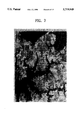
- FIG. 7 is gray scale photograph of the preferred embodiment using a Landsat thematic mapper image of bands 3, 4 and 5 of a wetland study area;
- FIG. 8 is a map of FIG. 7 based on a gray-scale image of Z-statistic values ranging between 0 and 255 where low values are dark while higher values are proportionally lighter;
- FIG. 9 is a map of FIG. 7 based on a generalized aerial photograph using the NWI classification system for the year 1982.
- FIG. 10 is the map of FIG. 7 based on the NWI classification system for 1992;
- FIG. 11 is a detailed map of FIGS. 9-10 showing the changes between 1982 and 1992 derived from comparing aerial images for both time frames;
- FIG. 12 is a map of FIG. 9-10 which represents a cross-correlation analysis map of the wetland changes resulting from the ungrouped classes between 1982 and 1992.
- FIG. 1 shows the hardware arrangement for the image processing system according to the present invention.
- FIG. 1 illustrates a system for converting high resolution data, such as maps derived from aerial photographs, so that such data can be used in conjunction with lower resolution, cheaper and more current data, to evaluate certain phenomena and provide greater information to the analyst than either data set used alone.
- the preferred embodiment of the data processed by this invention relates to using NWI vector data described above as the high resolution data source, and Landsat Thematic Mapper imagery as the low resolution data source.
- NWI vector data described above as the high resolution data source
- Landsat Thematic Mapper imagery Landsat Thematic Mapper imagery
- FIG. 1 illustrates an apparatus 10 for converting maps derived from high resolution data to a format which makes it possible to compare them to low resolution data pixel-by-pixel. (A pixel is the smallest data element of the low resolution data set.)
- the apparatus 10 includes a high resolution database 12 which can store either digital or digitized representations of analog objects to be analyzed.
- the aerial image data are archived as interpretive maps derived from aerial photos, as is done conventionally in the art.
- the aerial images are loaded into the database 12 as digital line graph ("DLG”) data.
- DDG digital line graph
- controller 16 which is adapted to coordinate, control, monitor and execute commands necessary for operating the low and high resolution input devices of FIGS. 1 and 2, as well as the cross-correlation unit of FIG. 3.
- controller 16 can comprise any appropriate microprocessor or minicomputer control device including, but not limited to, a PC-based controller or a dedicated control machine.
- the controller can comprise software implemented as a control program.
- a Solbourne NE UNIX-based minicomputer is used.
- the Solbourne has a 128 MIPS processor, 256 Kbytes of RAM and 40 gigabytes on hard drive.
- the Solbourne supports twelve terminals, a CIRRUS film recorder, three digital plotters, five digitizing tablets, and four laser printers.
- the controller 16 provides commands relating to the input, conversion, and read-out of the high resolution data in database 12. Moreover, the controller 16 is responsible for coordinating the operations of the downstream hardware.
- the database 12 is connected to an attribute memory 14.
- the purpose of the attribute memory is to store appropriate coding classifications that will be used in conjunction with the high resolution data contained in the database 12, and with the low resolution data stored in a separate memory that is shown in FIG. 2.
- the attribute memory 14 stores a classification code for wetlands which is based on a unique numeric code assigned to each wetland class.
- any classification scheme can be used, depending upon the type of application.
- the land use classification system developed by Anderson et al. (See U.S. Geol. Surv. Proj. Pap. 964) or the Florida Land Use Classification System, (see Florida Land Use and Form Classification System. Dept. of Transportation, State Topographic Bureau, Thematic Mapping Section,) can be used.
- a single wetland map may have over two hundred different types of wetlands where each type of wetland is a unique combination of system, subsystem, class, subclass and modifiers for a given habitat.
- the numeric coding scheme in the present invention assigns a particular wetland classification to each polygon of the high resolution NWI map and the low resolution thematic mapper image.
- the classification is conducted down to at least the subclass level.
- the classification scheme is based upon the aforedescribed work by Cowardin et al., Classification of Wetlands in Deepwater Habitats of the United States, U.S. Department of Interior, Fish and Wildlife Service, December 1979.
- the classification scheme converts the Cowardin taxa noted above into an eight bit code that defines the wetland system, subsystem class, subclass, and modifier which are exemplified below as chart 1.0.
- the code would be E1OWL and an integer value of 2 would be assigned to this wetland class.
- a chart of the exemplified study area classification definitions is provided below:
- the classification data (hereinafter NWI data) are interpreted in a manner which associates the NWI data with an interpreted vector of the high resolution data.
- NWI data The classification data
- the high resolution data are vectorized to conform to study parameters.
- vectorizing means identifying wetlands, and then segregating the discrete areas of the wetland which have identifiable characteristics.
- the vectorizing process typically creates polygons. If this process is done manually, then an overlay is created which is designed to be placed over the aerial photograph. If this process is done automatically, as in the present system, then an appropriate designation as described by the production facility is produced to represent the polygon.
- the second interpretation step involves assigning the attribute data 14 to the polygons.
- the assignment process may be done manually by having the operator create another overlay that corresponds to the vectors.
- the attributes can be attached automatically using a code/addressing algorithm for the vectors.
- at least two hundred different NWI classification types are coded. When more than 255 wetland types are found in a study area, the "most" similar types of classification are coded to have the same numeric value.
- Non-wetlands (such as uplands) are assigned a value of zero or may be assigned another value higher than the last wetland assignment.
- the data In order to assign proper attributes to each high resolution data set, the data must be converted into cells or units of uniform size.
- the DLG high resolution data are converted into polygonal vectors by a converter 18.
- the conversion process employs standard techniques for translation from most standard vector formats to the polygonal vector format used by the system.
- the preferred converter is the Arc Info conversion routine sold by Environmental Systems Research Institute, of Redlands, Calif.
- the conversion 18 involves rasterizing the derived DLG data by the raster device 22.
- the device 22 in turn is a conventional hardware raster or is a rasterizer program such as Arc Info module, "Polygrid”®.
- Arc Info module "Polygrid”®.
- a rasterized line of data is sent to the shift register 24 which is then stored in the high resolution vector memory 26.
- the functions of the shift register 24 can also be implemented by appropriate computer software. As a consequence, each raster line can be separately encoded and separately addressed in the high resolution vector memory via controller 16.
- the first process 32 involves determining the mean and standard deviation values of the low resolution data for each class value of the high resolution data set.
- a standard deviation and mean value processor 32 is controlled by the controller 16 and is connected to the high resolution vector memory 26.
- NWI classes are selected so that a sufficient sample size exists in order that accurately calculated mean, minimum, maximum and standard deviation values for the low resolution data using the resolution data as the zones occurs.
- NWI classes are also stored in the pixel classification memory 28.
- the cross-correlation routine has been implemented in ELAS, ERDAS, and Arc/Info.
- the first implementation was within ELAS.
- ELAS is a raster-based image processing software system that was initially developed by NASA. Many of the functions of cross-correlation analysis can be implemented within ELAS, but other functions of cross-correlation could not be implemented without adding additional functions to ELAS. To prototype the system, these required additional functions were re-created using the FORTRAN language. However, these FORTRAN models were external to ELAS and made the performance of cross-correlation awkward and inefficient.
- ERDAS External FORTRAN modules.
- ERDAS is a commercially available image processing software system which can be purchased from ERDAS of Atlanta, Ga. Cross-correlation could not be fully implemented within ERDAS using the existing modules. Other FORTRAN modules were written, but this implementation of the cross-correlation procedures had the same limitations of the ELAS implementation.
- Arc/Info a commercial GIS software system created and distributed by Environmental System Research Institute (ESRI) of Redlands, Calif.
- ESRI Environmental System Research Institute
- the cross-correlation procedures were implemented within Arc/Info using only existing Arc/Info modules and required no additional external programming.
- Arc/Info has its own programming language called Arc/Info Macro Language (AML) and cross-correlation was implemented by writing an AML for the entire process. No additional modules had to be created.
- AML Arc/Info Macro Language
- the data for wetland class 2 has mean values of 66, 24, 18, 11, 7 and 3 for Landsat TM bands 1, 2, 3, 4, 5 and 7 respectively.
- the minimum values for the Landsat scene for the NWI classification, E1OWL are 59, 18, 12, 3, 0 and 0 and the maximum values are 125, 72, 83, 133, 136 and 82.
- the standard deviations for E1OWL are defined for the following bands as being 5, 4, 5, 9, 12 and 5. These data are based on a total of 72,440 Landsat pixels for NWI class 2.
- the hardware arrangement 200 comprises a low resolution data memory 210 containing the low resolution pixel representations.
- these pixels are LANDSAT thematic mapper data.
- the pixels are stored in the memory so that each pixel is separately addressable.
- cross-correlated individual pixels may be required for small wetland areas.
- the Landsat TM signals provide seven spectral bands of information. Of the seven bands, band six is not selected from the satellite vector information by the selector 212. Only the optimum bands for the desired cross correlation are selected.
- the selector 212 can be programmed to by-pass or select those bands identified as either being unnecessary or as being important to the process.
- band 5 (1.55-1.75 um) has traditionally been considered the single most important band for its ability to discriminate levels of vegetation and moisture in the soil.
- Band 4 (0.76-0.90 um) is also important with respect to classifying vegetated communities and vegetation moisture. These data are helpful for inferring the existence of wetlands.
- band 3 (visible green) is valuable for measuring and defining deviations on a cell by cell basis (pixel-by-pixel).
- the geo-referencing processor 214 can comprise a conventional processor programmed with commercially available geo-referencing software, or specialized hardware. A variety of geo-referencing programs and techniques may be employed by processor 214. For example, a Global Positioning System (GPS) may be used to precisely locate each pixel or polygon. The advantage of using GPS is that it tends to produce a lower root mean square (RMS) error. However, in the preferred embodiment, a low resolution to high resolution data correction process is used so that the satellite image is accurately geo-referenced to the sub-pixel level. As a consequence, there is minimal displacement artificial between data sets. To avoid numerical problems with a polynomial approach, as well as to remove dominant errors, ephemeris data are used to correct to smaller errors (such as clock errors and space-craft-instrument misalignment).
- GPS Global Positioning System
- RMS root mean square
- the satellite image is rectified by unit 216 based upon the geometric correction value coefficient. Details of the rectification process performed by unit 216 are set forth in FIG. 5.
- the resulting rectified low resolution map image is then re-sampled by a rasterizer or other appropriate device to the chosen cell size. For example, in the preferred embodiment, a 25 by 25 meter-sized pixel cell is used (FIG. 4).
- the rasterized image lines are then stored in the low resolution image memory 219 for later use.
- FIG. 3 illustrates a detailed block-diagram of the two-pass cross-correlation apparatus forming a part of the present invention.
- FIG. 3 illustrates the two pass cross-correlation between the desired classes of the high resolution data and the brightness values of the low resolution data.
- the Z-statistic can be calculated as shown below: ##EQU1## where:
- C j is the assign class number derived from the high resolution data
- C max is the maximum number of classes from the high resolution data to be processed
- n is the number of bands of the low resolution data used
- i is a counter from one to n
- O i is the brightness value of the cell for the ith band of the low resolution data
- M ij is the mean of the brightness values for band i of the low resolution data and data C j of the high resolution data
- SD ij is the standard deviation of the brightness values for band i of the low resolution data and class C j of the high resolution data
- SF is a scale factor used. SF is chosen to increase the mean value of the calculated Z-statistic to be approximately 128.
- a memory 310 is provided for storing the pixel values of the low resolution data and the corresponding cell value of the class derived from the high resolution data.
- the mean and standard deviation for each of the wetland class delineated from the high resolution data are computed. These mean and standard deviations are computed for each of one of the wetland classes during the first pass of this cross-correlation routine.
- the calculation apparatus for the first pass is shown in FIG. 1.
- a Z-statistic value is created for each pixel in the study area.
- the Z-statistic is zero (0) for all cells not identified as wetland from the NWI maps derived from the high resolution data.
- the Z-statistic value can be set to reflect the characteristics that are desired to be measured, and set to zero for those that are not measured. This is processed by the class comparator 311. That is, if for the pixel being processed, the class value is zero (0) or greater than the maximum class value (max), then the Z-statistic is zero (0).
- the Z-statistic is computed by first subtracting the observed brightness value for a band (O i ) from the mean brightness value (M ij ) for bank (i) and class (j), where class (j) is the class value for the pixel being processed.
- the difference between the mean brightness value for a band and a class, and the observed brightness value, of a band for the pixel, is obtained in the subtractor unit 312.
- the divider 314 then divides this difference from subtractor 312 by the standard deviation previously calculated for band i and class j, where class j is the class for the pixel being processed.
- the above process normalized each difference in the observed and expected values for each mean. These normalized differences are then added together to derive an accumulated measure of deviation for each particular cell (pixel). This is done by the adder 318.
- the accumulated value is then multiplied in unit 316 by a scalar.
- the scalar is selected to distribute the Z-statistic between 0 and 255 with a mean of approximately 126.
- the resulting statistic is then compared to an a-priori threshold. The comparison is made by the comparator 320, with the threshold value, and is stored in memory 322.
- Z-statistics that are less than 90 may also be of interest. It was found that Z-statistic values between 50 and 90 may indicate potentially changed areas that require further investigation. In the preferred embodiment, where Z-statistics between 50 and 90 were found for areas, it appears that there either may have been (1) errors initially made in mapping those areas or, (2) the errors in the wetland typed had changed, only marginally, but the area still remained a wetland. Thus, the threshold memory typically would discriminate three separate categories: (1) statistical scores greater than 90 that indicate areas with significant changes, (2) statistical scores between 50 and 90 that indicate potential areas of change that require further evaluation, and (3) statistical scores of less than 50 that delineate areas that have had little or no detectable changes. Thresholds can obviously be varied depending upon the type of phenomena being evaluated.
- a change value derived from the comparator 320 is then provided to an appropriate printer/plotter device 326 or display 324 to show the designated areas of change. Detailed illustrations of these maps or displays are shown in FIGS. 7-12.
- step 402 the ingestion of high resolution data routine is initiated.
- the high resolution data 404 are loaded into the memory step 406, the data in the memory are converted into appropriate polygons.
- a conversion program can be used for this task.
- the aforementioned Arc Info module can accomplish this step.
- An unique attribute list is then built.
- there are typically over 200 unique wetland types such that, at step 408, each of the unique types are assigned a code.
- the vector codes are then compared to the wetland group attributes as identified in Table 1.1. If a match exists, then the appropriate integer image code is assigned at step 417.
- the integer code can be the NWI classification scheme. In the event that a match is not found, an error statement is produced, and the erroneous data are corrected. The corrected vector file is processed in step 404.
- all non-wetland polygons are assigned a zero value at step 417.
- the memory is then accessed to determine whether all vectors have been processed at step 408. If not, then the process loops back at step 426 to step 414 to compare to the attribute table. Once the loop is completed, the resulting polygons are loaded into the rasterizer 430 and a raster scan of the vector line then proceeds at step 432.
- the raster image of high resolution data that is fully attributed by the high resolution code, is loaded into memory 438. Accurately co-registering the low resolution data and the high resolution data is critical to the success of detecting true changes with this cross-correlation procedure and not detecting and reporting false changes. Falsely reported changes are termed commission errors.
- the source for low resolution data is usually satellite data, i.e. Landsat Thematic Mapper data
- the informational source for the high resolution data is generally vector data derived from aerial photography. Satellite data, because it is collected from a very stable platform in space, can usually be geocoded (georeferenced) to map projections with great precision. The positional accuracy of features derived from satellite data is usually very good. However, aerial photography is collected at much lower altitudes than satellite data and with an unstable base (i.e.
- FIG. 5 illustrates the procedures used to co-register the low and high resolution data sets.
- the accuracy of the co-registration is also appraised.
- Knowledge of the accuracy of the co-registration of the low and high resolution data sets is critical in interpreting the final results of this cross-correlation procedure.
- a buffer equal in length to the co-registration error is produced from the edge of all features mapped on the high resolution data. All changes detected within this buffered area may not be real and may be strictly the result of the error in registration of the two data sets.
- the co-registration 500 of the low resolution data to the high resolution data is illustrated.
- the routine 500 begins with step 502 where the low and high resolution data are loaded into memory 502 and the appropriate bands of low resolution data are selected.
- step 506 ephemeris data on the position of the satellite are pulled for use in creating the correction coefficients.
- the ephemeris data can only provide positional accuracy within a kilometer for Landsat data.
- ground control points must be selected from topographic maps and the locations of these points within the low resolution of the image must be identified 510.
- a correction coefficient is calculated 512 and the accuracy of the correction coefficient is tested on the ground control points 514.
- a priori accuracy standard i.e. 30 meters for Landsat Thematic Mapper data
- loop 518 sends the process back to 510 where additional control points are selected.
- the 518 loop to 510 to 516 is repeated until the a priori positional accuracy standard is met.
- the low resolution data are resampled to the appropriate cell size and projected to the desired projection system 520.
- the vectors of the high resolution data are then merged with the geocoded low resolution data 522.
- the positional accuracy of the co-registered data sets is ascertained in step 524.
- the geocoded low resolution data can be shifted at 528 to improve the co-registration of the data sets. If the final displacement is still significant as determined by step 530, a buffer is created that identifies the areas for which high Z-statistics are likely to be computed--not because of actual change, but because of the displacement between the low and high resolution data sets. This buffer will be used to identify areas for which confidence of detection-true change is low. The best geocoded data set that can be produced is then loaded into image memory for the Z-statistic calculations 534.
- FIG. 6 illustrates the steps used in the cross-correlation technique.
- the cross-correlation technique 600 is entered at step 602.
- This technique employs a two-pass process through the low resolution and high resolution data sets.
- the first pass steps 604-616
- the informational classes derived from the high resolution data are characterized by the low resolution image data.
- the mean brightness value and the standard deviation of the mean brightness value are calculated for each selected band of the low resolution image data.
- a Z-statistic is computed from the brightness values of the pixels from the low resolution image data and the mean and standard deviation of the brightness value of the informational class for the pixel.
- High Z values identify pixels that have changed between the time that the high resolution data were collected and the time that the low resolution data were collected.
- step 604 the next band of the low resolution data to be processed is selected.
- step 606 the next informational class derived from the high resolution data source to be processed is selected.
- Step 608 selects all pixels for the low resolution band being processed that are assigned the selected informational class derived from the high resolution data source.
- the mean brightness value for the selected band and class are calculated in step 610 and the standard deviation of the brightness value for the selected band and class are calculated in step 612.
- step 614 determines if the mean and standard deviation for all classes for the selected band have been processed. If not, the next class to be processed is determined in step 606. If the mean and standard deviation for all classes have been processed, the technique proceeds to step 616 to determine if all bands have been processed.
- the technique selects the next band for processing 604 and continues the above process. If all bands have not been processed, the technique selects the next band for processing 604 and continues the above process. If the mean and standard deviation have been calculated for all classes and all bands, the procedure begins the second pass through the low and high resolution data to ascertain the Z-statistic for each pixel. This second pass begins at step 618.
- Step 618 begins the pixel-by-pixel processing steps to calculate a Z-statistic for each pixel.
- step 618 the brightness values of all bands of the low resolution data and the class value derived from the high resolution data are obtained for the next pixel to be processed.
- Step 620 the normalized differences between the mean brightness values for the class value of the pixel and the observed brightness values are calculated. The normalized difference is calculated by calculating the difference between the observed brightness value and the mean brightness value, dividing this difference by the standard deviation, and squaring this value. This normalized difference is calculated for each band of low resolution data being processed.
- step 622 the normalized difference for each band processed is accumulated for all of the selected bands.
- Step 624 This accumulated normalized difference is then multiplied by the selected scalar in step 624 to calculate the final Z-statistic for each pixel.
- the scalar is selected to adjust the Z-statistic values so that the majority of Z-statistic values will range in value from 0 to 255.
- Step 626 the calculated Z-statistic is compared with an a priori threshold. If the Z-statistic for a pixel exceeds this threshold, then the pixel is used to map the detected change in step 632.
- Step 628 determines if all pixels have been processed. If all pixels have not been processed, the procedure loops back to step 618 and begins the pixel processing for the next pixel. When all pixels have been processed, the procedure ends.
- FIGS. 7, 8, 9, 10, 11 and 12 each represent different stages of the image processed by the instant invention in the preferred embodiment.
- FIG. 7 represents a gray scaled Thematic mapper image covering a study area.
- This image uses bands 3, 4 and 5 (filmed to green, red and blue respectively).
- the same area is then presented in FIG. 8 as a gray scaled image. Low values are shown as darker shades of gray while the higher values are proportionally lighter.
- the Z-statistic ranges in value in this image from 0 to 255.
- the 1982 generalized NWI classification system for the study area in FIGS. 7-8 is shown in FIG. 9.
- FIG. 10 shows the 1992 NWI classification for the study area.
- the detailed changes between the 1982 and 1992 high resolution analyses (aerial photography) for the study area are shown in FIG. 11.
- FIG. 12 An illustration of the results of the cross-correlation analysis of the wetlands change system applying the thresholds derived from the NWI classes is shown in FIG. 12.
- the present invention is not limited to the classification of wetlands data. Instead, it can also be used as a classification or change detector with any available low resolution data and may be used for classification of land use and land cover, including oceans and other water bodies.
- the present invention can be used to verify the initial NWI classification of wetlands.
- a Landsat TM scene is acquired for approximately the same date that the high resolution aerial photography was acquired.
- the Landsat TM imagery serves as the low resolution data and the aerial photogaphy serves as the high resolution data.
- the objective of this application is not to detect changes in wetlands that have occurred over time (since the sources of data were acquired at approximately the same time), but to verify the positional accuracy of the vectors derived from the aerial photography that maps and classifies the wetlands and the consistency of the classification of the wetlands.
- High Z-statistics under this application indicate positional accuracy errors or inconsistencies in the classification.
- this invention provides a quality control step for the initial NWI mapping that is very economical. Another example of how the system is used is for monitoring global change. Monitoring global change is a priority for NASA. As part of NASA's "Mission to Planet Earth", over $11 billion will be spent on the deployment of new satellites to monitor global change.
- This invention can be used with currently available satellite data and the new satellite systems proposed to aid in monitoring global change.
- forests can be mapped in detail using Landsat TM scenes. Changes to the forests can be effectively monitored by this invention.
- the vector data on the location and type of forests would be obtained from the Landsat data. These vectors would be compared to low resolution, less expensive, satellite data and changes (forest losses) could be delineated.
- AVHRR LAC data (with a spatial resolution of 1.1 km) could serve as the inexpensive source of low resolution data for monitoring global forest changes.
- this invention can be used in a cost effective manner to: monitor agricultural expansion, monitor urban expansion, monitor range land loses, monitor forest loses, identify areas of forest degradation (by disease, insects, or fire), identify losses of submerged aquatic vegetation, and monitor natural disasters.
Abstract
Description
                                  CHART 1
__________________________________________________________________________
        Wetland
Wetland Number
Class   Assigned
             System
                  Subsystem
                       Class    Subclass
                                        Modifiers
__________________________________________________________________________
E1ABLxns
        1    Estuarine
                  Subtidal
                       Aquatic Bed      Excavated, Mineral, Spoil
E1OWL   2    Estuarine
                  Subtidal
                       Open Water       Subtidal
E1OWL6  3    Estuarine
                  Subtidal
                       Open Water       Subtidal, Oligohaline
E1OWL6  4    Estuarine
                  Subtidal
                       Open Water       Subtidal, Oligohaline,
                                        Excavated
E1OWL   5    Estuarine
                  Subtidal
                       Open Water       Subtidal, Excavated
E1UB4L  6    Estuarine
                  Subtidal
                       Unconsolidated
                                Organic Subtidal
                       Bottom
E1UB4L6 7    Estuarine
                  Subtidal
                       Unconsolidated
                                Organic Subtidal, Oligohaline
                       Bottom
E1UB4L6X
        8    Estuarine
                  Subtidal
                       Unconsolidated
                                Organic Subtidal, Oligohaline,
                       Bottom           Excavated
E1UB4LX 9    Estuarine
                  Subtidal
                       Unconsolidated
                                Organic Subtidal, Excavated
                       Bottom
E1UB4Lx 10   Estuarine
                  Subtidal
                       Unconsolidated
                                Organic Subtidal, Excavated
                       Bottom
E1UBL   11   Estuarine
                  Subtidal
                       Unconsolidated   Subtidal
                       Bottom
E1UBLH  11   Estuarine
                  Subtidal
                       Unconsolidated   Subtidal, Diked/Impounded
                       Bottom
E1UBL6  12   Estuarine
                  Subtidal
                       Unconsolidated   Subtidal, Oligohaline
                       Bottom
E1UBL6X 13   Estuarine
                  Subtidal
                       Unconsolidated   Subtidal, Oligohaline,
                       Bottom           Excavated
E1UBLX  14   Estuarine
                  Subtidal
                       Unconsolidated   Subtidal, Excavated
                       Bottom
E1UBLx  15   Estuarine
                  Subtidal
                       Unconsolidated   Subtidal, Excavated
                       Bottom
E1USN   16   Estuarine
                  Subtidal
                       Unconsolidated   Regularly Flooded
                       Shore
E2AB2P6 17   Estuarine
                  Intertidal
                       Aquatic Bed
                                Submergent
                                        Irregularly Flooded, Oligohaline
                                vascular
E2ABN   18   Estuarine
                  Intertidal
                       Aquatic Bed      Regularly Flooded
E2ABP   19   Estuarine
                  Intertidal
                       Aquatic Bed      Irregularly Flooded
E2ABP6  20   Estuarine
                  Intertidal
                       Aquatic Bed      Irregularly Flooded, Oligohaline
E2EM/SS1P
        21   Estuarine
                  Intertidal
                       Emergent/Shrub-
                                /Broad-Leaved
                                        Irregularly Flooded
                       Scrub    Deciduous
E2EM1/SS1P6
        21   Estuarine
                  Intertidal
                       Emergent/Shrub-
                                Persistent/Broad-
                                        Irregularly Flooded, Oligohaline
                       Scrub    Leaved
                                Deciduous
E2EM1/FO5P
        22   Estuarine
                  Intertidal
                       Emergent/Forested
                                Persistent/Dead
                                        Irregularly Flooded
E2EM1N  23   Estuarine
                  Intertidal
                       Emergent Persistent
                                        Regularly Flooded
E2EM1NX 23   Estuarine
                  Intertidal
                       Emergent Persistent
                                        Regularly Flooded, Excavated
E2EM1Nns
        24   Estuarine
                  Intertidal
                       Emergent Persistent
                                        Regularly Flooded, Mineral,
                                        Spoil
E2EM1P  25   Estuarine
                  Intertidal
                       Emergent Persistent
                                        Irregularly Flooded
E2EM1Ph 25   Estuarine
                  Intertidal
                       Emergent Persistent
                                        Irregularly Flooded,
                                        Diked/Impounded
E2EM1P6 26   Estuarine
                  Intertidal
                       Emergent Persistent
                                        Irregularly Flooded, Oligohaline
E2EM1P6d
        26   Estuarine
                  Intertidal
                       Emergent Persistent
                                        Irregularly Flooded,
                                        Oligohaline, Partially
                                        Drained/Ditched
E2EM1Pdpub(w
        27   Estuarine
                  Intertidal
                       Emergent Persistent
                                        Irregularly Flooded, Partially
                                        Drained/Ditched, ****
E2EM1P  28   Estuarine
                  Intertidal
                       Emergent Persistent
                                        Irregularly Flooded, Spoil,
                                        Alkaline, Artificial Substrate
E2EM1U  29   Estuarine
                  Intertidal
                       Emergent Persistent
                                        Unknown
E2EM1Uh 29   Estuarine
                  Intertidal
                       Emergent Persistent
                                        Unknown, Diked/Impounded
E2EM1U6 30   Estuarine
                  Intertidal
                       Emergent Persistent
                                        Unknown, Oligohaline
E2EM1Usir
        31   Estuarine
                  Intertidal
                       Emergent Persistent
                                        Unknown, Spoil, Alkaline,
                                        Artificial Substrate
E2EM2N6 32   Estuarine
                  Intertidal
                       Emergent Nonpersistent
                                        Regularly Flooded, Oligohaline
E2EM5/2N6
        33   Estuarine
                  Intertidal
                       Emergent Nonpersistent/
                                        Regularly Flooded, Oligohaline
                                Narrow-leaved
E2EM5/FLN6
        34   Estuarine
                  Intertidal
                       Emergent/Flat
                                Persistent
                                Nonpersistent/
                                        Regularly Flooded, Oligohaline
                                Narrow-leaved
                                Persistent
E2EM5N  35   Estuarine
                  Intertidal
                       Emergent Nonpersistent/
                                        Regularly Flooded
                                Narrow-leaved
                                Persistent
E2EM5P  36   Estuarine
                  Intertidal
                       Emergent Nonpersistent/
                                        Irregularly Flooded
                                Narrow-leaved
                                Persistent
E2EM5P6 37   Estuarine
                  Intertidal
                       Emergent Nonpersistent/
                                        Irregularly Flooded, Oligohaline
                                Narrow-leaved
                                Persistent
E2EM5Pd 38   Estuarine
                  Intertidal
                       Emergent Nonpersistent/
                                        Irregularly Flooded, Partially
                                Narrow-leaved
                                        Drained/Ditched
                                Persistent
E2FLM   39   Estuarine
                  Intertidal
                       Flat             Irregularly Exposed
E2FLN   40   Estuarine
                  Intertidal
                       Flat             Regularly Flooded
E2FLN6  41   Estuarine
                  lntertidal
                       Flat             Regularly Flooded,
__________________________________________________________________________
                                        Oligohaline
                                  CHART 1.1
__________________________________________________________________________
INF CLS CLASS
        PIXELS
            CH 1  CH 2  CH 3  CH 4  CH 5  CH 6
                                             CH
__________________________________________________________________________
-2      72440
            66 (-42)
                  24 (-6)
                        18 (-7)
                              11 (-4)
                                    7  (-4)
                                          3
        MIN:
            59    18    12    3     0     0
        MAX:
            125   72    83    133   136   82
        STD:
            5     4     5     9     12    5
-3      23696
            68 (-41)
                  27 (-3)
                        24 (-12)
                              12 (-5)
                                    7  (-4)
                                          3
        MIN:
            62    22    17    5     0     0
        MAX:
            94    47    54    93    89    53
        STD:
            2     2     3     6     8     4
-4      37  73 (-44)
                  29 (-1)
                        28 (6)
                              34 (0)
                                    34 (-20)
                                          14
        MIN:
            63    24    21    21    15    7
        MAX:
            78    32    31    54    64    28
        STD:
            4     2     2     7     10    4
-5      32  78 (-45)
                  33 (0)
                        33 (17)
                              50 (13)
                                    63 (-38)
                                          25
        MIN 68    24    21    20    23    7
        MAX:
            98    46    53    81    116   47
        STD:
            6     4     7     14    21    9
-6      22  73 (-43)
                  30 (0)
                        30 (8)
                              38 (11)
                                    49 (-29)
                                          20
        MIN:
            68    26    25    20    24    9
        MAX:
            78    34    35    74    77    34
        STD:
            3     2     3     13    17    7
-7      18  74 (-44)
                  30 (0)
                        30 (21)
                              51 (11)
                                    62 (-35)
                                          27
        MIN:
            65    21    19    28    25    13
        MAX:
            86    42    48    85    98    44
        STD:
            5     5     7     14    17    8
-8      3   75 (-42)
                  33 (-4)
                        29 (88)
                              117
                                 (-38)
                                    79 (-51)
                                          28
        MIN:
            70    31    25    113   73    24
        MAX:
            83    37    35    120   89    31
        STD:
            6     3     4     3     7     3
-9      48  76 (-45)
                  31 (0)
                        31 (17)
                              48 (15)
                                    63 (-37)
                                          26
        MIN:
            67    23    17    16    15    6
        MAX:
            101   48    59    87    106   54
        STD:
            5     4     6     17    21    9
-10     8   87 (-47)
                  40 (6)
                        46 (12)
                              58 (29)
                                    87 (-37)
                                          50
        MIN:
            71    28    28    35    61    31
        MAX:
            98    50    64    74    117   74
        STD:
            10    8     13    15    20    16
-11     137201
            68 (-44)
                  24 (-4)
                        20 (-9)
                              11 (-3)
                                    8  (-4)
                                          4
        MIN:
            60    18    14    3     0     0
        MAX:
            127   57    70    88    134   78
        STD:
            3     3     4     6     13    6
-12     4330
            67 (-44)
                  23 (-2)
                        21 (-1)
                              20 (-4)
                                    16 (-9)
                                          7
        MIN:
            60    18    15    9     1     0
        MAX:
            92    42    47    86    101   48
        STD:
            3     3     4     9     13    6
-13     59  75 (-44)
                  31 (0)
                        31 (6)
                              37 (8)
                                    45 (-23)
                                          22
        MIN:
            67 25    22    13    6     3
        MAX:
            94    42    52    84    101   56
        STD:
            5     4     6     16    21    11
-14     369 77 (-46)
                  31 (1)
                        32 (12)
                              44 (17)
                                    61 (-35)
                                          26
        MIN:
            67    23    19    19    19    7
        MAX:
            134   72    87    99    149   80
        STD:
            8     6     8     11    19    10
-15     3   86 (-47)
                  39 (0)
                        39 (34)
                              73 (9)
                                    82 (-46)
                                          36
        MIN:
            82    35    34    49    59    24
        MAX:
            93    44    45    87    104   47
__________________________________________________________________________
Claims (9)
Priority Applications (1)
| Application Number | Priority Date | Filing Date | Title |
|---|---|---|---|
| US08/605,625 US5719949A (en) | 1994-10-31 | 1996-02-22 | Process and apparatus for cross-correlating digital imagery |
Applications Claiming Priority (2)
| Application Number | Priority Date | Filing Date | Title |
|---|---|---|---|
| US33227494A | 1994-10-31 | 1994-10-31 | |
| US08/605,625 US5719949A (en) | 1994-10-31 | 1996-02-22 | Process and apparatus for cross-correlating digital imagery |
Related Parent Applications (1)
| Application Number | Title | Priority Date | Filing Date |
|---|---|---|---|
| US33227494A Continuation | 1994-10-31 | 1994-10-31 |
Publications (1)
| Publication Number | Publication Date |
|---|---|
| US5719949A true US5719949A (en) | 1998-02-17 |
Family
ID=23297512
Family Applications (1)
| Application Number | Title | Priority Date | Filing Date |
|---|---|---|---|
| US08/605,625 Expired - Lifetime US5719949A (en) | 1994-10-31 | 1996-02-22 | Process and apparatus for cross-correlating digital imagery |
Country Status (1)
| Country | Link |
|---|---|
| US (1) | US5719949A (en) |
Cited By (45)
| Publication number | Priority date | Publication date | Assignee | Title |
|---|---|---|---|---|
| US5862245A (en) * | 1995-06-16 | 1999-01-19 | Alcatel Alsthom Compagnie Generale D'electricite | Method of extracting contours using a combined active contour and starter/guide approach |
| US6005961A (en) * | 1996-11-04 | 1999-12-21 | Samsung Electronics Co., Ltd. | Method for processing name when combining numerical map shape data |
| US6012016A (en) * | 1997-08-29 | 2000-01-04 | Bj Services Company | Method and apparatus for managing well production and treatment data |
| US6118885A (en) * | 1996-06-03 | 2000-09-12 | Institut Francais Du Petrole | Airborne image acquisition and processing system with variable characteristics |
| US6167144A (en) * | 1997-11-05 | 2000-12-26 | Mitsubishi Denki Kabushiki Kaisha | Image processing apparatus and image processing method for identifying a landing location on the moon or planets |
| US6243483B1 (en) * | 1998-09-23 | 2001-06-05 | Pii North America, Inc. | Mapping system for the integration and graphical display of pipeline information that enables automated pipeline surveillance |
| US20010026270A1 (en) * | 2000-03-29 | 2001-10-04 | Higgins Darin Wayne | System and method for synchronizing raster and vector map images |
| US20010033290A1 (en) * | 2000-03-29 | 2001-10-25 | Scott Dan Martin | System and method for georeferencing digial raster maps |
| US6345108B1 (en) * | 1997-12-10 | 2002-02-05 | Institut Francais Du Petrole | Multivariable statistical method for characterizing images that have been formed of a complex environment such as the subsoil |
| US6373995B1 (en) * | 1998-11-05 | 2002-04-16 | Agilent Technologies, Inc. | Method and apparatus for processing image data acquired by an optical scanning device |
| US6408085B1 (en) * | 1998-07-22 | 2002-06-18 | Space Imaging Lp | System for matching nodes of spatial data sources |
| US6571242B1 (en) * | 2000-07-25 | 2003-05-27 | Verizon Laboratories Inc. | Methods and systems for updating a land use and land cover map using postal records |
| US20040034498A1 (en) * | 2002-08-13 | 2004-02-19 | Shah Mohammed Kamran | Grouping components of a measurement system |
| US20040051680A1 (en) * | 2002-09-25 | 2004-03-18 | Azuma Ronald T. | Optical see-through augmented reality modified-scale display |
| US20040068758A1 (en) * | 2002-10-02 | 2004-04-08 | Mike Daily | Dynamic video annotation |
| US20040066391A1 (en) * | 2002-10-02 | 2004-04-08 | Mike Daily | Method and apparatus for static image enhancement |
| US6757445B1 (en) | 2000-10-04 | 2004-06-29 | Pixxures, Inc. | Method and apparatus for producing digital orthophotos using sparse stereo configurations and external models |
| US20040169664A1 (en) * | 2001-09-06 | 2004-09-02 | Hoffman Michael T. | Method and apparatus for applying alterations selected from a set of alterations to a background scene |
| US20040208396A1 (en) * | 2002-11-25 | 2004-10-21 | Deutsches Zentrum Fur Luft- Und Raumfahrt E.V. | Process and device for the automatic rectification of single-channel or multi-channel images |
| US20050047641A1 (en) * | 2003-08-30 | 2005-03-03 | Peter Volpa | Method and apparatus for determining unknown magnetic ink characters |
| US20050073532A1 (en) * | 2000-03-29 | 2005-04-07 | Scott Dan Martin | System and method for georeferencing maps |
| EP1622087A1 (en) * | 2004-07-29 | 2006-02-01 | Imagerie stereo appliquee au relief S.A. | Automatic digital cartographic image production |
| US7058197B1 (en) * | 1999-11-04 | 2006-06-06 | Board Of Trustees Of The University Of Illinois | Multi-variable model for identifying crop response zones in a field |
| US20070035562A1 (en) * | 2002-09-25 | 2007-02-15 | Azuma Ronald T | Method and apparatus for image enhancement |
| US20070088507A1 (en) * | 2005-10-13 | 2007-04-19 | James Haberlen | Systems and methods for automating environmental risk evaluation |
| US20070116365A1 (en) * | 2005-11-23 | 2007-05-24 | Leica Geosytems Geiospatial Imaging, Llc | Feature extraction using pixel-level and object-level analysis |
| US20070124182A1 (en) * | 2005-11-30 | 2007-05-31 | Xerox Corporation | Controlled data collection system for improving print shop operation |
| US20070162195A1 (en) * | 2006-01-10 | 2007-07-12 | Harris Corporation | Environmental condition detecting system using geospatial images and associated methods |
| US20070162193A1 (en) * | 2006-01-10 | 2007-07-12 | Harris Corporation, Corporation Of The State Of Delaware | Accuracy enhancing system for geospatial collection value of an image sensor aboard an airborne platform and associated methods |
| US20070162194A1 (en) * | 2006-01-10 | 2007-07-12 | Harris Corporation, Corporation Of The State Of Delaware | Geospatial image change detecting system with environmental enhancement and associated methods |
| US20070253639A1 (en) * | 2006-05-01 | 2007-11-01 | The United States Of America As Represented By The Secretary Of The Navy | Imagery analysis tool |
| US20080140271A1 (en) * | 2006-01-10 | 2008-06-12 | Harris Corporation, Corporation Of The State Of Delaware | Geospatial image change detecting system and associated methods |
| US20090289837A1 (en) * | 2006-08-01 | 2009-11-26 | Pasco Corporation | Map Information Update Support Device, Map Information Update Support Method and Computer Readable Recording Medium |
| US20100100539A1 (en) * | 2008-10-16 | 2010-04-22 | Curators Of The University Of Missouri | Identifying geographic-areas based on change patterns detected from high-resolution, remotely sensed imagery |
| US20100289642A1 (en) * | 2001-06-01 | 2010-11-18 | Landnet Corporation | Identification, storage and display of land data on a website |
| US8369567B1 (en) * | 2010-05-11 | 2013-02-05 | The United States Of America As Represented By The Secretary Of The Navy | Method for detecting and mapping fires using features extracted from overhead imagery |
| CN103177255A (en) * | 2013-03-15 | 2013-06-26 | 浙江大学 | Intertidal zone extraction method based on multiresolution digital elevation model |
| US8542884B1 (en) * | 2006-11-17 | 2013-09-24 | Corelogic Solutions, Llc | Systems and methods for flood area change detection |
| US20130250104A1 (en) * | 2012-03-20 | 2013-09-26 | Global Science & Technology, Inc | Low cost satellite imaging method calibrated by correlation to landsat data |
| US20140212055A1 (en) * | 2013-01-25 | 2014-07-31 | Shyam Boriah | Automated Mapping of Land Cover Using Sequences of Aerial Imagery |
| US20180102034A1 (en) * | 2015-09-28 | 2018-04-12 | Dongguan Frontier Technology Institute | Fire disaster monitoring method and apparatus |
| CN108665489A (en) * | 2017-03-27 | 2018-10-16 | 波音公司 | The method and data processing system of variation for detecting geographical space image |
| US10255526B2 (en) | 2017-06-09 | 2019-04-09 | Uptake Technologies, Inc. | Computer system and method for classifying temporal patterns of change in images of an area |
| CN109635836A (en) * | 2018-11-09 | 2019-04-16 | 广西壮族自治区遥感信息测绘院 | Remote sensing image Forest road hierarchy detection method based on sparse DBN model |
| US20200279097A1 (en) * | 2017-09-13 | 2020-09-03 | Project Concern International | System and method for identifying and assessing topographical features using satellite data |
Citations (4)
| Publication number | Priority date | Publication date | Assignee | Title |
|---|---|---|---|---|
| US4364085A (en) * | 1980-04-22 | 1982-12-14 | Arvin Industries, Inc. | Colorized weather satellite converter |
| US4706296A (en) * | 1983-06-03 | 1987-11-10 | Fondazione Pro Juventute Don Carlo Gnocchi | Modularly expansible system for real time processing of a TV display, useful in particular for the acquisition of coordinates of known shape objects |
| US4984279A (en) * | 1989-01-04 | 1991-01-08 | Emyville Enterprises Limited | Image processing and map production systems |
| US5187754A (en) * | 1991-04-30 | 1993-02-16 | General Electric Company | Forming, with the aid of an overview image, a composite image from a mosaic of images |
-
1996
- 1996-02-22 US US08/605,625 patent/US5719949A/en not_active Expired - Lifetime
Patent Citations (4)
| Publication number | Priority date | Publication date | Assignee | Title |
|---|---|---|---|---|
| US4364085A (en) * | 1980-04-22 | 1982-12-14 | Arvin Industries, Inc. | Colorized weather satellite converter |
| US4706296A (en) * | 1983-06-03 | 1987-11-10 | Fondazione Pro Juventute Don Carlo Gnocchi | Modularly expansible system for real time processing of a TV display, useful in particular for the acquisition of coordinates of known shape objects |
| US4984279A (en) * | 1989-01-04 | 1991-01-08 | Emyville Enterprises Limited | Image processing and map production systems |
| US5187754A (en) * | 1991-04-30 | 1993-02-16 | General Electric Company | Forming, with the aid of an overview image, a composite image from a mosaic of images |
Non-Patent Citations (8)
| Title |
|---|
| Leib et al, "Aerial Reconnaissance Film Screening Using Optical Matched-Filter . . . " pp. 2892-2899 Sep. 1978. |
| Leib et al, Aerial Reconnaissance Film Screening Using Optical Matched Filter . . . pp. 2892 2899 Sep. 1978. * |
| Mattikalli, "An Integrated Geographical Information System's Approach . . . " Feb. 1994 pp. 1204-1206. |
| Mattikalli, An Integrated Geographical Information System s Approach . . . Feb. 1994 pp. 1204 1206. * |
| Takahashi et al. "LANDSAT Image Data Processing System" pp. 261-266 Oct. 1980. |
| Takahashi et al. LANDSAT Image Data Processing System pp. 261 266 Oct. 1980. * |
| Villasenor et al, "Change Detection on Alaska's North Slope . . . " pp. 227-236 Jan. 1993. |
| Villasenor et al, Change Detection on Alaska s North Slope . . . pp. 227 236 Jan. 1993. * |
Cited By (79)
| Publication number | Priority date | Publication date | Assignee | Title |
|---|---|---|---|---|
| US5862245A (en) * | 1995-06-16 | 1999-01-19 | Alcatel Alsthom Compagnie Generale D'electricite | Method of extracting contours using a combined active contour and starter/guide approach |
| US6118885A (en) * | 1996-06-03 | 2000-09-12 | Institut Francais Du Petrole | Airborne image acquisition and processing system with variable characteristics |
| US6005961A (en) * | 1996-11-04 | 1999-12-21 | Samsung Electronics Co., Ltd. | Method for processing name when combining numerical map shape data |
| US6012016A (en) * | 1997-08-29 | 2000-01-04 | Bj Services Company | Method and apparatus for managing well production and treatment data |
| US6167144A (en) * | 1997-11-05 | 2000-12-26 | Mitsubishi Denki Kabushiki Kaisha | Image processing apparatus and image processing method for identifying a landing location on the moon or planets |
| US6345108B1 (en) * | 1997-12-10 | 2002-02-05 | Institut Francais Du Petrole | Multivariable statistical method for characterizing images that have been formed of a complex environment such as the subsoil |
| US6408085B1 (en) * | 1998-07-22 | 2002-06-18 | Space Imaging Lp | System for matching nodes of spatial data sources |
| US6243483B1 (en) * | 1998-09-23 | 2001-06-05 | Pii North America, Inc. | Mapping system for the integration and graphical display of pipeline information that enables automated pipeline surveillance |
| US6373995B1 (en) * | 1998-11-05 | 2002-04-16 | Agilent Technologies, Inc. | Method and apparatus for processing image data acquired by an optical scanning device |
| US7058197B1 (en) * | 1999-11-04 | 2006-06-06 | Board Of Trustees Of The University Of Illinois | Multi-variable model for identifying crop response zones in a field |
| US7142217B2 (en) | 2000-03-29 | 2006-11-28 | Sourceprose Corporation | System and method for synchronizing raster and vector map images |
| US20010026271A1 (en) * | 2000-03-29 | 2001-10-04 | Higgins Darin Wayne | System and method for synchronizing raster and vector map images |
| US20010033290A1 (en) * | 2000-03-29 | 2001-10-25 | Scott Dan Martin | System and method for georeferencing digial raster maps |
| US20010028348A1 (en) * | 2000-03-29 | 2001-10-11 | Higgins Darin Wayne | System and method for synchronizing raster and vector map images |
| US20030052896A1 (en) * | 2000-03-29 | 2003-03-20 | Higgins Darin Wayne | System and method for synchronizing map images |
| US7038681B2 (en) | 2000-03-29 | 2006-05-02 | Sourceprose Corporation | System and method for georeferencing maps |
| US7161604B2 (en) | 2000-03-29 | 2007-01-09 | Sourceprose Corporation | System and method for synchronizing raster and vector map images |
| US7167187B2 (en) * | 2000-03-29 | 2007-01-23 | Sourceprose Corporation | System and method for georeferencing digital raster maps using a georeferencing function |
| US20010033291A1 (en) * | 2000-03-29 | 2001-10-25 | Scott Dan Martin | System and method for georeferencing digital raster maps |
| US20050073532A1 (en) * | 2000-03-29 | 2005-04-07 | Scott Dan Martin | System and method for georeferencing maps |
| US7190377B2 (en) | 2000-03-29 | 2007-03-13 | Sourceprose Corporation | System and method for georeferencing digital raster maps with resistance to potential errors |
| US7148898B1 (en) | 2000-03-29 | 2006-12-12 | Sourceprose Corporation | System and method for synchronizing raster and vector map images |
| US20010026270A1 (en) * | 2000-03-29 | 2001-10-04 | Higgins Darin Wayne | System and method for synchronizing raster and vector map images |
| US6571242B1 (en) * | 2000-07-25 | 2003-05-27 | Verizon Laboratories Inc. | Methods and systems for updating a land use and land cover map using postal records |
| US6757445B1 (en) | 2000-10-04 | 2004-06-29 | Pixxures, Inc. | Method and apparatus for producing digital orthophotos using sparse stereo configurations and external models |
| US20100289642A1 (en) * | 2001-06-01 | 2010-11-18 | Landnet Corporation | Identification, storage and display of land data on a website |
| US20040169664A1 (en) * | 2001-09-06 | 2004-09-02 | Hoffman Michael T. | Method and apparatus for applying alterations selected from a set of alterations to a background scene |
| US20040034498A1 (en) * | 2002-08-13 | 2004-02-19 | Shah Mohammed Kamran | Grouping components of a measurement system |
| US7002551B2 (en) | 2002-09-25 | 2006-02-21 | Hrl Laboratories, Llc | Optical see-through augmented reality modified-scale display |
| US20070035562A1 (en) * | 2002-09-25 | 2007-02-15 | Azuma Ronald T | Method and apparatus for image enhancement |
| US20040051680A1 (en) * | 2002-09-25 | 2004-03-18 | Azuma Ronald T. | Optical see-through augmented reality modified-scale display |
| US20040068758A1 (en) * | 2002-10-02 | 2004-04-08 | Mike Daily | Dynamic video annotation |
| US20040066391A1 (en) * | 2002-10-02 | 2004-04-08 | Mike Daily | Method and apparatus for static image enhancement |
| US7356201B2 (en) * | 2002-11-25 | 2008-04-08 | Deutsches Zentrum für Luft- und Raumfahrt e.V. | Process and device for the automatic rectification of single-channel or multi-channel images |
| US20040208396A1 (en) * | 2002-11-25 | 2004-10-21 | Deutsches Zentrum Fur Luft- Und Raumfahrt E.V. | Process and device for the automatic rectification of single-channel or multi-channel images |
| US20050047641A1 (en) * | 2003-08-30 | 2005-03-03 | Peter Volpa | Method and apparatus for determining unknown magnetic ink characters |
| US7474780B2 (en) | 2003-08-30 | 2009-01-06 | Opex Corp. | Method and apparatus for determining unknown magnetic ink characters |
| WO2006010623A1 (en) * | 2004-07-29 | 2006-02-02 | Imagerie Stereo Appliquee Au Relief S.A. | Automatic digital cartographic image production |
| EP1622087A1 (en) * | 2004-07-29 | 2006-02-01 | Imagerie stereo appliquee au relief S.A. | Automatic digital cartographic image production |
| US20070088507A1 (en) * | 2005-10-13 | 2007-04-19 | James Haberlen | Systems and methods for automating environmental risk evaluation |
| US20070116365A1 (en) * | 2005-11-23 | 2007-05-24 | Leica Geosytems Geiospatial Imaging, Llc | Feature extraction using pixel-level and object-level analysis |
| US7933451B2 (en) | 2005-11-23 | 2011-04-26 | Leica Geosystems Ag | Feature extraction using pixel-level and object-level analysis |
| US20070124182A1 (en) * | 2005-11-30 | 2007-05-31 | Xerox Corporation | Controlled data collection system for improving print shop operation |
| US9396445B2 (en) * | 2005-11-30 | 2016-07-19 | Xeroz Corporation | Controlled data collection system for improving print shop operation |
| US7630797B2 (en) * | 2006-01-10 | 2009-12-08 | Harris Corporation | Accuracy enhancing system for geospatial collection value of an image sensor aboard an airborne platform and associated methods |
| US20070162194A1 (en) * | 2006-01-10 | 2007-07-12 | Harris Corporation, Corporation Of The State Of Delaware | Geospatial image change detecting system with environmental enhancement and associated methods |
| US7528938B2 (en) | 2006-01-10 | 2009-05-05 | Harris Corporation | Geospatial image change detecting system and associated methods |
| US7603208B2 (en) * | 2006-01-10 | 2009-10-13 | Harris Corporation | Geospatial image change detecting system with environmental enhancement and associated methods |
| US20070162195A1 (en) * | 2006-01-10 | 2007-07-12 | Harris Corporation | Environmental condition detecting system using geospatial images and associated methods |
| US20080140271A1 (en) * | 2006-01-10 | 2008-06-12 | Harris Corporation, Corporation Of The State Of Delaware | Geospatial image change detecting system and associated methods |
| US8433457B2 (en) * | 2006-01-10 | 2013-04-30 | Harris Corporation | Environmental condition detecting system using geospatial images and associated methods |
| US20070162193A1 (en) * | 2006-01-10 | 2007-07-12 | Harris Corporation, Corporation Of The State Of Delaware | Accuracy enhancing system for geospatial collection value of an image sensor aboard an airborne platform and associated methods |
| US20070253639A1 (en) * | 2006-05-01 | 2007-11-01 | The United States Of America As Represented By The Secretary Of The Navy | Imagery analysis tool |
| US20090289837A1 (en) * | 2006-08-01 | 2009-11-26 | Pasco Corporation | Map Information Update Support Device, Map Information Update Support Method and Computer Readable Recording Medium |
| US8138960B2 (en) * | 2006-08-01 | 2012-03-20 | Pasco Corporation | Map information update support device, map information update support method and computer readable recording medium |
| US8542884B1 (en) * | 2006-11-17 | 2013-09-24 | Corelogic Solutions, Llc | Systems and methods for flood area change detection |
| US20100100548A1 (en) * | 2008-10-16 | 2010-04-22 | Curators Of The University Of Missouri | Storing change features detected from high-resolution, remotely sensed imagery |
| US20100100539A1 (en) * | 2008-10-16 | 2010-04-22 | Curators Of The University Of Missouri | Identifying geographic-areas based on change patterns detected from high-resolution, remotely sensed imagery |
| US20100100540A1 (en) * | 2008-10-16 | 2010-04-22 | Curators Of The University Of Missouri | Revising imagery search results based on user feedback |
| US8156136B2 (en) | 2008-10-16 | 2012-04-10 | The Curators Of The University Of Missouri | Revising imagery search results based on user feedback |
| US8243997B2 (en) * | 2008-10-16 | 2012-08-14 | The Curators Of The University Of Missouri | Detecting geographic-area change using high-resolution, remotely sensed imagery |
| US8250481B2 (en) | 2008-10-16 | 2012-08-21 | The Curators Of The University Of Missouri | Visualizing geographic-area change detected from high-resolution, remotely sensed imagery |
| US20100098342A1 (en) * | 2008-10-16 | 2010-04-22 | Curators Of The University Of Missouri | Detecting geographic-area change using high-resolution, remotely sensed imagery |
| US9514386B2 (en) | 2008-10-16 | 2016-12-06 | The Curators Of The University Of Missouri | Identifying geographic areas based on change patterns detected from high-resolution, remotely sensed imagery |
| US20100100835A1 (en) * | 2008-10-16 | 2010-04-22 | Curators Of The University Of Missouri | Visualizing geographic-area change detected from high-resolution, remotely sensed imagery |
| US8001115B2 (en) | 2008-10-16 | 2011-08-16 | The Curators Of The University Of Missouri | Identifying geographic-areas based on change patterns detected from high-resolution, remotely sensed imagery |
| US8369567B1 (en) * | 2010-05-11 | 2013-02-05 | The United States Of America As Represented By The Secretary Of The Navy | Method for detecting and mapping fires using features extracted from overhead imagery |
| US20130250104A1 (en) * | 2012-03-20 | 2013-09-26 | Global Science & Technology, Inc | Low cost satellite imaging method calibrated by correlation to landsat data |
| US20140212055A1 (en) * | 2013-01-25 | 2014-07-31 | Shyam Boriah | Automated Mapping of Land Cover Using Sequences of Aerial Imagery |
| US8958603B2 (en) * | 2013-01-25 | 2015-02-17 | Regents Of The University Of Minnesota | Automated mapping of land cover using sequences of aerial imagery |
| CN103177255B (en) * | 2013-03-15 | 2016-01-20 | 浙江大学 | A kind of intertidal zone extraction method based on multiresolution digital elevation model |
| CN103177255A (en) * | 2013-03-15 | 2013-06-26 | 浙江大学 | Intertidal zone extraction method based on multiresolution digital elevation model |
| US20180102034A1 (en) * | 2015-09-28 | 2018-04-12 | Dongguan Frontier Technology Institute | Fire disaster monitoring method and apparatus |
| CN108665489A (en) * | 2017-03-27 | 2018-10-16 | 波音公司 | The method and data processing system of variation for detecting geographical space image |
| CN108665489B (en) * | 2017-03-27 | 2023-03-21 | 波音公司 | Method for detecting changes in geospatial images and data processing system |
| US10255526B2 (en) | 2017-06-09 | 2019-04-09 | Uptake Technologies, Inc. | Computer system and method for classifying temporal patterns of change in images of an area |
| US20200279097A1 (en) * | 2017-09-13 | 2020-09-03 | Project Concern International | System and method for identifying and assessing topographical features using satellite data |
| US11587310B2 (en) * | 2017-09-13 | 2023-02-21 | Project Concern International | System and method for identifying and assessing topographical features using satellite data |
| CN109635836A (en) * | 2018-11-09 | 2019-04-16 | 广西壮族自治区遥感信息测绘院 | Remote sensing image Forest road hierarchy detection method based on sparse DBN model |
Similar Documents
| Publication | Publication Date | Title |
|---|---|---|
| US5719949A (en) | Process and apparatus for cross-correlating digital imagery | |
| Lunetta et al. | Remote sensing and geographic information system data integration- Error sources and research issues | |
| Malila | Change vector analysis: An approach for detecting forest changes with Landsat | |
| Congalton | Remote sensing and geographic information system data integration: error sources and | |
| Liu et al. | Object-based shadow extraction and correction of high-resolution optical satellite images | |
| Bernstein | Digital image processing of earth observation sensor data | |
| Haralick | Automatic remote sensor image processing | |
| US7505608B2 (en) | Methods and apparatus for adaptive foreground background analysis | |
| Matikainen et al. | Automatic detection of buildings from laser scanner data for map updating | |
| Baltsavias | Digital ortho-images—a powerful tool for the extraction of spatial-and geo-information | |
| CN107527328B (en) | Unmanned aerial vehicle image geometric processing method considering precision and speed | |
| CN112712535B (en) | Mask-RCNN landslide segmentation method based on simulation difficult sample | |
| Kauth et al. | Blob: An unsupervised clustering approach to spatial preprocessing of mss imagery | |
| Gallaudet et al. | Automated cloud screening of AVHRR imagery using split-and-merge clustering | |
| Kouchi et al. | Characteristics of tsunami-affected areas in moderate-resolution satellite images | |
| JP2001143054A (en) | Satellite image-processing method | |
| Gastellu-Etchegorry | An assessment of SPOT XS and Landsat MSS data for digital classification of near-urban land cover | |
| Mohamed et al. | Change detection techniques using optical remote sensing: a survey | |
| Swann et al. | The potential for automated mapping from geocoded digital image data | |
| Coulter et al. | Comparison of high spatial resolution imagery for efficient generation of GIS vegetation layers | |
| Carlotto | Spectral shape classification of Landsat Thematic Mapper imagery | |
| Schiek | Terrain change detection using ASTER optical satellite imagery along the Kunlun fault, Tibet | |
| Defoe | Considerations in the Design of a System for the Rapid Acquisition of Geographic Information | |
| Data | Band-moment analysis of imaging-spectrometer data | |
| Kandoba et al. | The system for automated deciphering of cosmic Earth surface photographs |
Legal Events
| Date | Code | Title | Description |
|---|---|---|---|
| STCF | Information on status: patent grant |
Free format text: PATENTED CASE |
|
| FPAY | Fee payment |
Year of fee payment: 4 |
|
| FPAY | Fee payment |
Year of fee payment: 8 |
|
| FPAY | Fee payment |
Year of fee payment: 12 |
|
| AS | Assignment |
Owner name: EARTH SATELLITE CORPORATION, MARYLAND Free format text: ASSIGNMENT OF ASSIGNORS INTEREST;ASSIGNOR:KOELN, GREGORY T;REEL/FRAME:027709/0185 Effective date: 19950110 |
|
| AS | Assignment |
Owner name: MDA INFORMATION SYSTEMS, INC., MARYLAND Free format text: CHANGE OF NAME;ASSIGNOR:MDA FEDERAL INC.;REEL/FRAME:028222/0913 Effective date: 20091208 Owner name: MDA FEDERAL INC., MARYLAND Free format text: CHANGE OF NAME;ASSIGNOR:EARTH SATELLITE CORPORATION;REEL/FRAME:028222/0679 Effective date: 20050718 |
|
| AS | Assignment |
Owner name: MDA INFORMATION SYSTEMS LLC, MARYLAND Free format text: MERGER;ASSIGNOR:MDA INFORMATION SYSTEMS, INC.;REEL/FRAME:034583/0363 Effective date: 20120831 |
|
| AS | Assignment |
Owner name: ROYAL BANK OF CANADA, AS THE COLLATERAL AGENT, CANADA Free format text: SECURITY INTEREST;ASSIGNORS:DIGITALGLOBE, INC.;MACDONALD, DETTWILER AND ASSOCIATES LTD.;MACDONALD, DETTWILER AND ASSOCIATES CORPORATION;AND OTHERS;REEL/FRAME:044167/0396 Effective date: 20171005 Owner name: ROYAL BANK OF CANADA, AS THE COLLATERAL AGENT, CAN Free format text: SECURITY INTEREST;ASSIGNORS:DIGITALGLOBE, INC.;MACDONALD, DETTWILER AND ASSOCIATES LTD.;MACDONALD, DETTWILER AND ASSOCIATES CORPORATION;AND OTHERS;REEL/FRAME:044167/0396 Effective date: 20171005 |
|
| AS | Assignment |
Owner name: MAXAR SPACE LLC, CALIFORNIA Free format text: TERMINATION AND RELEASE OF SECURITY INTEREST IN PATENTS AND TRADEMARKS - RELEASE OF REEL/FRAME 044167/0396;ASSIGNOR:ROYAL BANK OF CANADA, AS AGENT;REEL/FRAME:063543/0001 Effective date: 20230503 Owner name: MAXAR INTELLIGENCE INC., COLORADO Free format text: TERMINATION AND RELEASE OF SECURITY INTEREST IN PATENTS AND TRADEMARKS - RELEASE OF REEL/FRAME 044167/0396;ASSIGNOR:ROYAL BANK OF CANADA, AS AGENT;REEL/FRAME:063543/0001 Effective date: 20230503 |