US8358233B2 - Radar target detection process - Google Patents
Radar target detection process Download PDFInfo
- Publication number
- US8358233B2 US8358233B2 US12/924,030 US92403010A US8358233B2 US 8358233 B2 US8358233 B2 US 8358233B2 US 92403010 A US92403010 A US 92403010A US 8358233 B2 US8358233 B2 US 8358233B2
- Authority
- US
- United States
- Prior art keywords
- vector
- target
- tilde over
- clean
- amplitude
- Prior art date
- Legal status (The legal status is an assumption and is not a legal conclusion. Google has not performed a legal analysis and makes no representation as to the accuracy of the status listed.)
- Expired - Fee Related, expires
Links
Images


Classifications
-
- G—PHYSICS
- G01—MEASURING; TESTING
- G01S—RADIO DIRECTION-FINDING; RADIO NAVIGATION; DETERMINING DISTANCE OR VELOCITY BY USE OF RADIO WAVES; LOCATING OR PRESENCE-DETECTING BY USE OF THE REFLECTION OR RERADIATION OF RADIO WAVES; ANALOGOUS ARRANGEMENTS USING OTHER WAVES
- G01S7/00—Details of systems according to groups G01S13/00, G01S15/00, G01S17/00
- G01S7/02—Details of systems according to groups G01S13/00, G01S15/00, G01S17/00 of systems according to group G01S13/00
- G01S7/28—Details of pulse systems
- G01S7/285—Receivers
- G01S7/292—Extracting wanted echo-signals
- G01S7/2921—Extracting wanted echo-signals based on data belonging to one radar period
Definitions
- the invention relates generally to improving range resolution of radar-illuminated targets.
- the invention enables the radar to detect and record data on a small target that could otherwise be obscured by larger targets.
- Pulse compression is achieved by modulating the radar pulse and then processing it with a matched filter on receiver.
- the response of the matched filter compresses the pulse to a width that can be reduced by the time-bandwidth product of the modulated pulse. This enables detection of two identical amplitude targets that can be spaced closer by the time-bandwidth product of the modulated pulse. Good modulation produces small sidelobes.
- FIG. 1 shows a graphical view 100 of a pulse received signal signal.
- the abscissa 110 represents time or range, and the ordinate 120 represents signal strength or amplitude. At the origin where time and range are zero, the amplitude reaches maximum extent denoted as an un-modulated pulse 130 orthogonal to the span 140 .
- a matched filter response 150 provides a linear rise across the span's extent.
- a pulse-compression matched filter response 160 to the modulated pulse exhibits a narrower extent across the span 140 than for the un-modulated, with sidelobes 170 disposed adjacent thereto.
- sidelobes can interfere with the detection of small targets in the presence of large targets.
- FIG. 2 shows a graphical view 200 of a secondary signal.
- the abscissa 210 represents time or range, and the ordinate 220 represents signal strength or amplitude.
- the pulse-compression matched filter response 160 can be compared against a second target, which from compression includes a detectable response 230 and anon-detectable response 240 that remains obscured by the sidelobes 170 .
- various exemplary embodiments provide a process for analyzing a radar signal using CLEAN to identify an undetected target in sidelobes of a detected target.
- the process includes obtaining system impulse response data of a waveform for a point target having a signal data vector based on a convolution under conjugate transpose multiplied by a target amplitude vector plus a noise vector, estimating the target amplitude vector, and applying a CLEAN Deconvolver to remove the detected target from the data signal vector based on the estimate amplitude vector absent the detected target and an amplitude vector of an undetected target.
- the process further includes building a detected target vector with the amplitude estimate vector, setting to zero all elements of the detected target vector except at an initial time, and recomputing the amplitude estimate vector by a Reformulated CLEAN Detector.
- FIG. 1 is a graphical view of a primary compression signal
- FIG. 2 is a graphical view of a secondary compression signal
- FIG. 3 is a graphical view of a sinc plot
- FIG. 4 is a block diagram view of a radar system
- FIG. 5 is a graphical view of a Correlator output based on a filtered pulse
- FIG. 6 is a graphical view of a CLEAN Deconvolver output based on perfect calibration
- FIG. 7 is a graphical view of a CLEAN Deconvolver output based on estimated calibration
- FIG. 8 is a graphical view of a CLEAN Deconvolver output for small SNR targets
- FIG. 9 is a graphical view of a Reformulated CLEAN Detector output for small SNR targets.
- FIG. 10 is a block diagram view of a flowchart using the CLEAN Detector
- FIG. 11 is a graphical view of a CLEAN Correlator output for all targets
- FIG. 12 is a graphical view of a CLEAN Deconvolver output for high SNR targets
- FIG. 13 is a graphical view of a CLEAN Deconvolver output for a large target
- FIG. 14 is a graphical view of a CLEAN Detector output for small targets
- FIG. 15 is a graphical view of a CLEAN Deconvolver output for small targets
- FIG. 16 is a graphical view of a Correlator output for all targets with low SNR.
- FIG. 17 is a graphical view of a Reformulated CLEAN Detector output for small SNR targets.
- Radar designers normally operate their transmitters in a saturated condition to maximize the energy in the pulse. This means that modulations schemes are limited to phase modulated schemes.
- the second line of attack is replacing the matched filter with a filter that compresses the pulse and produce lower sidelobes. Although such filters are feasible to design, the matched filter is the optimum filter for detecting targets. Therefore, other filters are suboptimal, meaning that there causing a loss in detectability. Consequently, practical mismatched filters still face limitations on their sidelobe performance.
- CLEAN algorithm Another technique applied to this problem is the CLEAN algorithm.
- the CLEAN algorithm was developed by astronomers to increase the resolution of photographs of stars, being originally documented by J. A. Högbom: “Aperture Synthesis with a Non-Regular Distribution of Interferometer Baselines”, Astronomy and Astrophysics Supplement , v. 415, pp. 417-426.
- CLEAN works by subtracting the point spread function (PFS) of the brightest star.
- the PFS is the response to a point source.
- the PFS can be the response of the image due to the finite resolution of optics. This procedure is repeated with the remaining brightest source until the remaining scene is at the noise floor or some other predefined criteria.
- the amplitude and position of each source is noted and represents the Cleaned image.
- the point sources are convolved with the PFS minus the sidelobes to produce the Cleaned image.
- the process disclosed in exemplary embodiments employs an algorithm that assumes the entire radar listen interval has been band limited with a suitable bandpass filter, digitized and is available for processing.
- AWGN additive white Gaussian noise
- W ⁇ [ 0 ... 0 w t 0 ... w t 0 ⁇ w t ... 0 0 ] , ( 2 ) where w represents the vector of the impulse response of the transmitted waveform plus the receive chain, superscript t is the transpose operation.
- ⁇ ( ⁇ tilde over (W) ⁇ tilde over (W) ⁇ H ) ⁇ 1 ⁇ tilde over (W) ⁇ y, (3) where ⁇ is the minimum variance unbiased estimate of the target amplitude vector c.
- ⁇ coor ⁇ tilde over (W) ⁇ y, (4) where ⁇ corr represents the matched filter estimate.
- CLEAN algorithm involves three elements. First, the spectrum of the data can be controlled by proper selection of filtering and sample rate. The second element is obtaining the point spread function (PSF), also known as system impulse response. This is also called the calibration problem. The third element is applying combinations of the CLEAN Deconvolver, Correlator and CLEAN Detector, depending on signal-to-noise ratio (SNR) of the data and the quality of the PSF, to produce the best estimate of the target amplitude vector c.
- PSF point spread function
- SNR signal-to-noise ratio
- the first element is the least apparent part of this approach. This is due to considerations in the frequency-domain, while the entire deconvolution approach can be based completely on time-domain analysis.
- spectral shaping involves the operation of deconvolution in the time domain, which is equivalent to multiplying the reciprocal of the PSF Fourier transform times the Fourier transform of the received or observed data.
- y(t) represents the observed data
- h(t) is the impulse response of the radar
- c(t) is the target complex (i.e., collection or scatters)
- ⁇ (t) ⁇ - ⁇ ⁇ ⁇ Y ⁇ ( f ) H ⁇ ( f ) ⁇ e - j2 ⁇ ⁇ ⁇ ft ⁇ ⁇ d f , ( 7 )
- ⁇ (t) is the continuous time estimate of the target complex.
- y ( t ) h ( t ) ⁇ circle around (x) ⁇ ⁇ ( t ⁇ t 0 ), (8) where t 0 corresponds to the range of the target and ⁇ represents an impulse function.
- t 0 corresponds to the range of the target
- ⁇ represents an impulse function.
- ⁇ (t) constitutes a time-dependent sinc function of f 0 t obtained from the inverse Fourier transform by integrating over the bandwidth f 0 of the radar waveform.
- FIG. 3 shows a graphical view 300 for a Response of Deconvolution to a single point target.
- the abscissa 310 represents time or range, and the ordinate 320 represents amplitude.
- the normalized sinc function used for digital signal processing and communication may be expressed as:
- the second element is obtaining the PSF or impulse response of the radar. This represents an important aspect of applying the CLEAN algorithm, because any errors in determining the PSF can significantly degrade or destroy the performance of the CLEAN algorithm.
- the overall response of the system includes the radar transmitter, antenna, and receive path to the point that the baseband data are provided for processing and detection.
- FIG. 4 provides a block diagram of a radar system 400 .
- a waveform generator 410 generates a baseband signal s, which is converted to a carrier frequency at mixer 415 and processed through a band-pass filter 420 before being submitted to a transmitter 425 and emitted through a transmit antenna 430 as a propagating signal 435 aimed at a spherical target 440 , which reflects radiated energy as a reflected signal 445 .
- a receive antenna 450 captures the reflected signal 445 , which is processed through a band-pass filter 455 before gain is applied by a low noise amplifier 460 .
- the amplified signal is downconverted by a mixer 465 , run through a low-pass filter 470 , and digitized by an analog-to-digital (A/D) converter 475 to provide observed broadband data y as the output 480 .
- observed data vector y obtained from a point target such as the sphere 440 is the impulse response or PSF of the entire radar.
- observed data vector y 1 represents a column vector of length p
- convolution matrix ⁇ tilde over (S) ⁇ 1 has size of p ⁇ l
- impulse response h is a column vector of length l.
- the parameter l corresponds to the length of the impulse response of the radar, excluding the driving waveform vector s.
- p is the length of the total impulse of the radar including the driving waveform vector s.
- y 2 ⁇ tilde over (S) ⁇ 2 ( ⁇ tilde over (S) ⁇ 1 H ⁇ tilde over (S) ⁇ 1 ) ⁇ 1 ⁇ tilde over (S) ⁇ 1 H y 1 , (13) where y 2 is the second observed data vector adjusted by calibration from the first observed data vector y 1 .
- the impulse response (or PSF) is inferred from the second observed data vector y 2 .
- the third element is the application of the various forms of the CLEAN algorithm developed in the pervious Foreman papers, plus the reformulated CLEAN Detector described below. These processes are applied based on the properties of the observed data vector y. For data consisting of all uneclipsed targets, the process uses the CLEAN Deconvolver and reformulated CLEAN Detector, as in the 2007 Foreman paper.
- target Doppler can preferably be taken into account. As described in the 2006 Foreman paper, uncompensated target Doppler destroys the performance of the CLEAN Deconvolver and CLEAN Detector. Therefore, the Doppler for high SNR targets in the scene should preferably be determined or estimated if unknown, and included in the CLEAN algorithms.
- the CLEAN Deconvolver should be used for the detection of all high SNR uneclipsed targets, as described in eqn. (3). This resolves targets to the nearest range sample.
- the range-time sidelobe performance of the CLEAN Deconvolver can be determined by the selection of filter and sampling rate, as discussed in element-1 and the SNR of the calibration data from element-2.
- the CLEAN Deconvolver can be used in conjunction with the correlator to detect the large targets. This can be accomplished by subjecting the vector ⁇ in eqn. (3) to a threshold test that determines which elements have targets that can be detected by the CLEAN Deconvolver.
- the correlator combined with the Reformulated CLEAN Detector should be applied. This is accomplished by first determining the location and amplitude of all the large targets, and may be performed with the CLEAN Deconvolver provided the target SNRs are sufficient. The correlator can be used for low SNR targets.
- the next step is to build the large target vector c + by including the amplitude estimates of the large targets detected. Every other element of large target vector c + is set to zero.
- the final step is to compute in eqn.
- noise amplitude is assumed to be unity
- I is an identity matrix of the noise amplitude
- the elements of c are evaluated against a threshold to detect previous undetected small targets.
- c + vector of large targets
- FIG. 5 illustrates a graphical view 500 for Correlator Output based on a filtered pulse, with the target in the center.
- the plot shows time/range representing the abscissa 510 and SNR in decibels (dB) as the ordinate 520 .
- PSK phase shift keying
- the range time sidelobes are only 17 dB down from the peak of the target response. In this example, the Range-Time sidelobes prevent detecting smaller targets.
- FIG. 6 illustrates a graphical view 600 for CLEAN Output based on perfect calibration, with the target in the center.
- the plot shows frequency representing the abscissa 610 and SNR in dB as the ordinate 620 .
- the output signal 630 of shows the performance possible with a measured PSF at high SNR.
- the target, indicated by the sharp pulse signal 640 is localized to a single range cell and Range-Time sidelobes are over 90 dB down from the peak of the target response. This demonstrates the importance of the first element of this methodology, namely controlling the frequency spectrum and sampling rate. In addition this demonstrates the importance of having a PSF measurement with high SNR.
- FIG. 7 illustrates a graphical view 700 for CLEAN Deconvolver Output based on estimated calibration, with the target in the center.
- the plot shows range-time representing the abscissa 710 and SNR in dB as the ordinate 720 .
- the output signal 730 is based on synthesizing the PSF for a different phase code from the measured PSF associated with the perfect calibration plot 600 , with attendant degradation of the range-time sidelobes by comparison.
- the CLEAN Deconvolver is the preferred process for sufficient SNR.
- FIG. 8 shows a graphical view 800 of a CLEAN Deconvolver Output for small SNR targets.
- This plot 800 shows range-time representing the abscissa 810 and SNR in dB as the ordinate 820 .
- the output signal 830 exhibits considerable noise that obscures secondary targets.
- the final example is the application of the Reformulated CLEAN Detector.
- the same target complex was simulated with a much lower SNR.
- the CLEAN Deconvolver could not detect the largest target. This is illustrated in CLEAN Output plot 800 .
- the SNR of the large target is 11 dB while the SNR of the three small targets is ⁇ 4 dB.
- FIG. 9 shows a graphical view 900 of a Reformulated CLEAN Detector output for small SNR targets.
- This plot 900 shows range-time representing the abscissa 910 and SNR in dB as the ordinate 920 .
- the three smaller targets 930 can clearly be seen since the large target has been removed. This is contrast to 500 and 800 in which the small targets could not be seen.
- FIG. 10 shows a block diagram view 1000 of a flowchart with the process of applying the CLEAN algorithm technique for detecting a small target.
- the process begins at step 1010 for each radar waveform to be evaluated.
- a query 1020 determines whether calibration data are available for the waveform. If so, the process collects data 480 at step 1030 from the point-like spherical target 440 (as indicated in the block diagram 400 ).
- the observed data 480 provide the impulse function or PSF of the radar. If data are unavailable, then the PSF may be synthesized at step 1140 to apply eqn. (13) from a single measurement of PSF (i.e., for an alternate available waveform). Note that improved performance results from high SNR values.
- the process continues to control the frequency response and sampling rate at step 1050 .
- the PSF in the frequency domain multiplied by the convolution filter response can be set to unity over the sampling rate ⁇ f 0 or written 1/(2f 0 ) This can be verified by applying the CLEAN Deconvolver to the calibration data, such as in plot 600 . Low range-time sidelobes in the signal 630 indicate that the calibration data are valid, and that the frequency response and sampling rate have been properly controlled.
- the CLEAN Deconvolver and Detector may be applied to detect or measure amplitude of targets, depending on the SNR of the various targets. If all targets of interest have high SNR, then the CLEAN Deconvolver or else the CLEAN Detector can be used to provide maximum amplitude measurement accuracy and resolution performance.
- the process then stops at step 1070 for that waveform, and returns to the initial step 1010 if evaluating another waveform.
- FIG. 11 shows a graphical view 1100 of a second example performance results.
- This plot 1100 shows range-time representing the abscissa 1110 and SNR in dB as the ordinate 1120 .
- the signal 1130 obscures all but the maximum target indicated by spike 1140 .
- the matched filter or correlator provides the maximum output SNR for additive white noise.
- the plot 1100 shows the output of a hypothetical radar using a 32-chip derivative phase shift keying waveform with the each chip repeated sixteen times, similar to plot 500 .
- the range time sidelobes are only 17 dB down from the peak of the target response.
- a large center target has 35 dB SNR, whereas by contrast and three smaller ones has only 26 dB SNR. Only the large target can be reliably detected at spike 1140 due to the range-time sidelobes of the waveform used.
- FIG. 12 shows a graphical view 1200 with the same data processed by the CLEAN Deconvolver.
- This plot 1200 shows range-time representing the abscissa 1210 and SNR in dB as the ordinate 1220 .
- the target peaks 1240 can be observed.
- all four targets are distinguishable, showing the strength of the Deconvolver such that targets can be localized to a single range cell.
- the targets are not injected at the range cell boundaries, but instead are disposed in straddling range cells by oversampling the input data and then filtering and down-sampling.
- FIG. 13 shows a graphical view 1300 of the effect of additional noise.
- the smaller targets have such low SNR at 12 dB that they can not be seen with the CLEAN Deconvolver.
- This plot 1300 shows range-time representing the abscissa 1310 and SNR in dB as the ordinate 1320 .
- the signal 1330 obscures all but the largest spike 1340 .
- the noise prevents the detection of the smaller targets.
- the correlator also fails to detect the smaller targets due to the range-time sidelobes of the waveform. Here, only the largest target can be observed as the spike 1340 by the CLEAN Deconvolver.
- FIG. 14 shows a graphical view 1400 for the Reformulated CLEAN Detector used to detect the smaller targets.
- This plot 1400 shows range-time representing the abscissa 1410 and SNR in dB as the ordinate 1420 .
- the signal 1430 shows three spikes 1440 .
- the Reformulated CLEAN Detector has the effect of eliminating (i.e., occluding) the large target detected by the CLEAN Deconvolver.
- the three smaller targets are detected as spikes 1430 with virtually no interference from the large target.
- only the largest targets can be observed by the CLEAN Deconvolver.
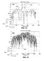
- FIG. 15 shows a graphical view 1500 of a situation to be analyzed in which the larger target has SNR too low to be detectable by the CLEAN Deconvolver.
- the larger target SNR is 8 dB while the three smaller targets have a SNR of ⁇ 9 dB.
- This plot 1500 shows range-time representing the abscissa 1510 and SNR in dB as the ordinate 1520 .
- the Output of the CLEAN Deconvolver renders the large target undetectable, shown as signal 1530 .
- the SNR of the large target is too small to enable detection by the CLEAN Deconvolver.
- FIG. 16 shows a graphical view 1600 of an Output of the Correlator in which the largest target is detected.
- This plot 1600 shows range-time representing the abscissa 1610 and SNR in dB as the ordinate 1620 .
- the signal 1630 indicates the presence of the largest target by its accompanying spike 1640 .
- the correlator has higher gain than the CLEAN Detector in the presence of noise, the correlator can detect the larger target.
- This is shown in plot 1600 , in which Output of the Correlator shows the large target detected by the spike 1640 . Because the larger target can be detected by the correlator in plot 1600 , the amplitude and position of the target can be estimated by the correlator.
- FIG. 17 shows a graphical view 1700 from estimation by the correlator using the Reformed CLEAN Detector.
- This plot 1700 shows range-time representing the abscissa 1710 and SNR in dB as the ordinate 1720 .
- the signal 1730 also reveals three spikes 1740 indicating the smaller targets subsequent to occlusion of the largest target.
- the Reformulated CLEAN Detector in plot 1700 can detect the three smaller targets.
- Various exemplary embodiments enable very low sidelobes for the detection of closely spaced targets with largely differing amplitudes.
- Other various embodiments alternatively or additionally provide for significantly improved resolution with waveforms that would otherwise have poor range resolution.
- Advantages include improved range resolution performance with existing radars by only changing the signal processing and leaving the waveform generator, transmitter chain and receiver chain intact.
- amplitude estimation accuracy is improved because this process includes a practical implementation of a minimum variance unbiased estimator.
- Another advantage is improved detection of low signal to noise ratio (SNR) targets in the presence of large signal to noise ratio targets by simultaneously maximizing the SNR of the small targets and minimizing the SNR from previously detected large targets.
- SNR signal to noise ratio
- a further advantage is improved target length estimates.
- waveforms are not constrained to be minimum phase.
Abstract
Description
- (1) R. Bose: “Sequence CLEAN Technique Using BGA for Contiguous Radar Target Images with High Sidelobes”, IEEE Transactions on Aerospace and Electronic Systems, v. 39, no. 1, pp 368-373, January 2003;
- (2) I.-S. Choi and H.-T. Kim: “One-dimensional Evolutionary Programming-based CLEAN”, Electronics Letters, v. 37, no. 6, 15 Mar. 2001;
- (3) R. Bose, A. Freedman, and B. D. Steinberg: “Sequence CLEAN: A Modified Deconvolution Technique for Microwave Images of Contiguous Targets”, IEEE Transactions on Aerospace and Electronic Systems, v. 38, no 1, January 2002; and
- (4) H. Deng: “Effective CLEAN Algorithms for Performance-Enhanced Detection of Binary Coding Radar Signals”, IEEE Transactions on Signal Processing, v. 52, no. 1, January 2004.
y={tilde over (W)} H c+n, (1)
where y represents the received observation data, {tilde over (W)} represents the convolution operation, superscript H is conjugate transpose operation, c is the vector of target amplitudes, and n is a vector of additive white Gaussian noise (AWGN). Multiplication by {tilde over (W)} represents the operation of convolution as an array such that:
where w represents the vector of the impulse response of the transmitted waveform plus the receive chain, superscript t is the transpose operation.
- (5) T. L. Foreman: “Adapting the CLEAN Deconvolver and CLEAN Detector to Doppler Uncertainty”, IEEE Radar Conference, 2007; and
- (6) T. L. Foreman: “Reinterpreting the CLEAN Algorithm as an Optimum Detector”, IEEE Radar Conference, April 2006.
ĉ=({tilde over (W)}{tilde over (W)} H)−1 {tilde over (W)}y, (3)
where ĉ is the minimum variance unbiased estimate of the target amplitude vector c. By contrast, a matched filter would yield:
ĉ coor ={tilde over (W)}y, (4)
where ĉcorr represents the matched filter estimate.
y(t)=h(t){circle around (x)}c(t), (5)
where {circle around (x)} is the convolution operator between the impulse response and the target complex (of scatters).
Y(f)=H(f)·C(f), (6)
where such convolution in the Fourier transforms domain is replaced by multiplication.
where ĉ(t) is the continuous time estimate of the target complex.
y(t)=h(t){circle around (x)}δ(t−t 0), (8)
where t0 corresponds to the range of the target and δ represents an impulse function. When the range is arbitrarily set to t0=0, in the limit observed frequency transform Y(f) approaches the value impulse response transform H(f), such as the ratio Y(f)÷H(f) becomes unity, the Fourier transform of eqn. (8) can be incorporated into eqn. (7) to obtain:
where ĉ(t) constitutes a time-dependent sinc function of f0t obtained from the inverse Fourier transform by integrating over the bandwidth f0 of the radar waveform.
in which the sinc function of eqn. (10) equals unity at the x=0 singularity) and has a rectangular Fourier transform.
y 1 ={tilde over (S)} 1 h, (11)
where h is the impulse response of the system separate of the driving waveform s1 (output of 410 of
where elements si are the elements of driving waveform vector s1 from i=1, 2, . . . p.
y 2 ={tilde over (S)} 2({tilde over (S)} 1 H {tilde over (S)} 1)−1 {tilde over (S)} 1 H y 1, (13)
where y2 is the second observed data vector adjusted by calibration from the first observed data vector y1.
where
where noise amplitude is assumed to be unity, I is an identity matrix of the noise amplitude, and the elements of
Claims (6)
y={tilde over (W)} H c+n,
ĉ=({tilde over (W)}{tilde over (W)} H)−1 {tilde over (W)}y,
y 1 ={tilde over (S)} 1 h,
y 2 ={tilde over (S)} 2({tilde over (S)} 1 H {tilde over (S)} 1)−1 {tilde over (S)} 1 H y 1,
Priority Applications (1)
| Application Number | Priority Date | Filing Date | Title |
|---|---|---|---|
| US12/924,030 US8358233B2 (en) | 2009-09-14 | 2010-09-14 | Radar target detection process |
Applications Claiming Priority (2)
| Application Number | Priority Date | Filing Date | Title |
|---|---|---|---|
| US27718509P | 2009-09-14 | 2009-09-14 | |
| US12/924,030 US8358233B2 (en) | 2009-09-14 | 2010-09-14 | Radar target detection process |
Publications (2)
| Publication Number | Publication Date |
|---|---|
| US20120313805A1 US20120313805A1 (en) | 2012-12-13 |
| US8358233B2 true US8358233B2 (en) | 2013-01-22 |
Family
ID=47292724
Family Applications (1)
| Application Number | Title | Priority Date | Filing Date |
|---|---|---|---|
| US12/924,030 Expired - Fee Related US8358233B2 (en) | 2009-09-14 | 2010-09-14 | Radar target detection process |
Country Status (1)
| Country | Link |
|---|---|
| US (1) | US8358233B2 (en) |
Cited By (1)
| Publication number | Priority date | Publication date | Assignee | Title |
|---|---|---|---|---|
| US9201141B1 (en) * | 2012-07-13 | 2015-12-01 | Lockheed Martin Corporation | Multiple simultaneous transmit track beams using phase-only pattern synthesis |
Families Citing this family (5)
| Publication number | Priority date | Publication date | Assignee | Title |
|---|---|---|---|---|
| KR102584888B1 (en) * | 2016-07-29 | 2023-10-06 | 한국전자통신연구원 | Apparatus and method for detecting radar signal |
| CN109959934B (en) * | 2017-12-26 | 2023-02-17 | 中国船舶重工集团公司七五〇试验场 | Method for detecting underwater buried target by multi-beam high resolution |
| CN109507664B (en) * | 2019-01-22 | 2020-05-22 | 中国人民解放军空军工程大学 | Compressed sensing MIMO radar cognitive waveform obtaining method and device |
| CN110471036B (en) * | 2019-08-23 | 2022-08-02 | 电子科技大学 | False target cleaning method used in large array near field focusing |
| CN111273296B (en) * | 2020-02-27 | 2021-11-02 | 浙江工业大学 | Iterative deconvolution-time reversal target detection and distance estimation method |
Citations (14)
| Publication number | Priority date | Publication date | Assignee | Title |
|---|---|---|---|---|
| US4894660A (en) * | 1988-10-12 | 1990-01-16 | General Electric Company | Range sidelobe reduction by aperiodic swept-frequency subpulses |
| US4982150A (en) * | 1989-10-30 | 1991-01-01 | General Electric Company | Spectral estimation utilizing an autocorrelation-based minimum free energy method |
| US5068597A (en) * | 1989-10-30 | 1991-11-26 | General Electric Company | Spectral estimation utilizing a minimum free energy method with recursive reflection coefficients |
| US5351058A (en) | 1979-02-26 | 1994-09-27 | The United States Of America As Represented By The Secretary Of The Navy | General purpose sidelobe canceller system |
| US5361069A (en) | 1969-07-18 | 1994-11-01 | The United States Of America As Represented By The Secretary Of The Air Force | Airborne radar warning receiver |
| US5414428A (en) | 1993-08-06 | 1995-05-09 | Martin Marietta Corp. | Radar system with pulse compression and range sidelobe suppression preceding doppler filtering |
| US5570094A (en) * | 1995-10-10 | 1996-10-29 | Armstrong; Brian S. R. | Three dimensional tracking by array doppler radar |
| US5579011A (en) * | 1979-11-02 | 1996-11-26 | Grumman Aerospace Corporation | Simultaneous triple aperture radar |
| US5686922A (en) * | 1995-09-29 | 1997-11-11 | Environmental Research Institute Of Michigan | Super spatially variant apodization (Super - SVA) |
| US5781157A (en) | 1996-08-05 | 1998-07-14 | Mcdonnell Douglas Corporation | Multiple beam radar system with enhanced sidelobe supression |
| US6100844A (en) | 1994-06-15 | 2000-08-08 | Hollandse Signaalapparaten B.V. | Radar apparatus with sidelobe blanking circuit |
| US6268821B1 (en) | 1977-10-21 | 2001-07-31 | Raytheon Company | Multiple band sidelobe canceller |
| US6867726B1 (en) | 1991-12-16 | 2005-03-15 | Lockheed Martin Corporation | Combining sidelobe canceller and mainlobe canceller for adaptive monopulse radar processing |
| US20100134345A1 (en) * | 2008-11-28 | 2010-06-03 | Thales Nederland B.V. | Method for filtering a radar signal after it has been reflected by a target |
-
2010
- 2010-09-14 US US12/924,030 patent/US8358233B2/en not_active Expired - Fee Related
Patent Citations (14)
| Publication number | Priority date | Publication date | Assignee | Title |
|---|---|---|---|---|
| US5361069A (en) | 1969-07-18 | 1994-11-01 | The United States Of America As Represented By The Secretary Of The Air Force | Airborne radar warning receiver |
| US6268821B1 (en) | 1977-10-21 | 2001-07-31 | Raytheon Company | Multiple band sidelobe canceller |
| US5351058A (en) | 1979-02-26 | 1994-09-27 | The United States Of America As Represented By The Secretary Of The Navy | General purpose sidelobe canceller system |
| US5579011A (en) * | 1979-11-02 | 1996-11-26 | Grumman Aerospace Corporation | Simultaneous triple aperture radar |
| US4894660A (en) * | 1988-10-12 | 1990-01-16 | General Electric Company | Range sidelobe reduction by aperiodic swept-frequency subpulses |
| US4982150A (en) * | 1989-10-30 | 1991-01-01 | General Electric Company | Spectral estimation utilizing an autocorrelation-based minimum free energy method |
| US5068597A (en) * | 1989-10-30 | 1991-11-26 | General Electric Company | Spectral estimation utilizing a minimum free energy method with recursive reflection coefficients |
| US6867726B1 (en) | 1991-12-16 | 2005-03-15 | Lockheed Martin Corporation | Combining sidelobe canceller and mainlobe canceller for adaptive monopulse radar processing |
| US5414428A (en) | 1993-08-06 | 1995-05-09 | Martin Marietta Corp. | Radar system with pulse compression and range sidelobe suppression preceding doppler filtering |
| US6100844A (en) | 1994-06-15 | 2000-08-08 | Hollandse Signaalapparaten B.V. | Radar apparatus with sidelobe blanking circuit |
| US5686922A (en) * | 1995-09-29 | 1997-11-11 | Environmental Research Institute Of Michigan | Super spatially variant apodization (Super - SVA) |
| US5570094A (en) * | 1995-10-10 | 1996-10-29 | Armstrong; Brian S. R. | Three dimensional tracking by array doppler radar |
| US5781157A (en) | 1996-08-05 | 1998-07-14 | Mcdonnell Douglas Corporation | Multiple beam radar system with enhanced sidelobe supression |
| US20100134345A1 (en) * | 2008-11-28 | 2010-06-03 | Thales Nederland B.V. | Method for filtering a radar signal after it has been reflected by a target |
Non-Patent Citations (11)
| Title |
|---|
| C.-F. Chang et al.: "Frequency Division Multiplexing Technique for Composite Ambiguity Function Approximation", Digital Signal Processing, 16, 5, 488-497, 2005. |
| H. Deng: "Effective Clean Algorithms for PerfOrmance-Enhanced Detection of Binary Coding Radar Signals", IEEE Transactions on Signal Processing, v. 52, No. 1, Jan. 2004. |
| I.-S. Choi et al.: "One-dimensional Evolutionary Programming-based CLEAN", Electronics Ltrs, 37, 6, Mar. 15, 2001. |
| J.A. Högbom: "Aperture Synthesis with a Non-Regular Distribution of Interferometer Baselines", Astronomy and Astrophysics Supplement, 415, 417-426, 1974. |
| Nelander, A.; , "Deconvolution approach to terrain scattered interference mitigation," Radar Conference, 2002. Proceedings of the IEEE , vol., no., pp. 344-349, 2002. * |
| R. Bose, et al.: "Sequence CLEAN: A Modified Deconvolution Technique for Microwave Images of Contiguous Targets", IEEE Trans. on Aerospace and Electronic Systems, 38, Jan. 1, 2002. |
| R. Bose: "Sequence CLEAN Technique Using BGA for Contiguous Radar Target Images with High Sidelobes", IEEE Trans. on Aerospace and Electronic Systems, 39, 1, 368-373, Jan. 2003. |
| See-May Phoong; Vaidyanathan, P.P.; , "One- and two-level filter-bank convolvers," Signal Processing, IEEE Transactions on , vol. 43, No. 1, pp. 116-133, Jan. 1995. * |
| Skinner, B.J.; Donohoe, J.P.; Ingels, F.M.; , "Simulation of target responses to high frequency ultra wideband radar signals using the physical optics impulse response," System Theory, 1993. Proceedings SSST '93., Twenty-Fifth Southeastern Symposium on , vol., no., pp. 11-15, Mar. 7-9, 1993. * |
| T.L. Foreman: "Adapting the CLEAN Deconvolver & CLEAN Detector to Doppler Uncertainty", IEEE Radar Conf., 2007. |
| T.L. Foreman: "Reinterpreting the CLEAN Algorithm as an Optimum Detector", IEEE Radar Conference, Apr. 2006. |
Cited By (1)
| Publication number | Priority date | Publication date | Assignee | Title |
|---|---|---|---|---|
| US9201141B1 (en) * | 2012-07-13 | 2015-12-01 | Lockheed Martin Corporation | Multiple simultaneous transmit track beams using phase-only pattern synthesis |
Also Published As
| Publication number | Publication date |
|---|---|
| US20120313805A1 (en) | 2012-12-13 |
Similar Documents
| Publication | Publication Date | Title |
|---|---|---|
| US10024958B2 (en) | Radar apparatus | |
| EP1672379B1 (en) | System and method for reducing a radar interference signal | |
| US8358233B2 (en) | Radar target detection process | |
| EP2097769B1 (en) | System and method for reducing the effect of a radar interference signal | |
| US5565764A (en) | Digital processing method for parameter estimation of synchronous, asynchronous, coherent or non-coherent signals | |
| EP2771710B1 (en) | Wideband sonar receiver and sonar signal processing algorithms | |
| JP6818541B2 (en) | Radar device and positioning method | |
| EP3211445A1 (en) | Radar system | |
| US11204410B2 (en) | Radar-based communication | |
| US11846696B2 (en) | Reduced complexity FFT-based correlation for automotive radar | |
| CN109061589A (en) | The Target moving parameter estimation method of random frequency hopping radar | |
| US6184820B1 (en) | Coherent pulse radar system | |
| US7248207B2 (en) | System and method for sidelobe reduction using point spread function expansion | |
| US6624783B1 (en) | Digital array stretch processor employing two delays | |
| CN114609623B (en) | Target detection method and device of monopulse radar and computer equipment | |
| US7339519B2 (en) | Methods and apparatus for target radial extent determination using deconvolution | |
| US20130234878A1 (en) | System and Method of Radar Location | |
| US10386471B1 (en) | Velocity estimation with linear frequency modulated (LFM) waveforms | |
| Taylor | Ultra wideband radar | |
| Mir et al. | Low-rate sampling technique for range-windowed radar/sonar using nonlinear frequency modulation | |
| JP2015049074A (en) | Radar and object detection method | |
| CN110907930B (en) | Vehicle-mounted radar target detection and estimation method and device based on angle estimation | |
| US9429644B1 (en) | Subaperture clutter filter with CFAR signal detection | |
| KR101524550B1 (en) | Method and Apparatus for a fast Linear Frequency Modulation target detection compensating Doppler effect according to the target speed | |
| Foreman | Application of the CLEAN detector to low signal to noise ratio targets |
Legal Events
| Date | Code | Title | Description |
|---|---|---|---|
| AS | Assignment |
Owner name: NAVY, UNITED STATES OF AMERICA REPRESENTED BY SEC. Free format text: ASSIGNMENT OF ASSIGNORS INTEREST;ASSIGNOR:FOREMAN, TERRY L.;REEL/FRAME:025195/0184 Effective date: 20100916 |
|
| AS | Assignment |
Owner name: NAVY, UNITED STATES OF AMERICA, REPRESENTED BY SEC Free format text: ASSIGNMENT OF ASSIGNORS INTEREST;ASSIGNOR:FOREMAN, TERRY L.;REEL/FRAME:025994/0470 Effective date: 20100916 |
|
| AS | Assignment |
Owner name: NAVY, UNITED STATES OF AMERICA, REPRESENTED BY SEC Free format text: CORRECTION OF PRIOR RECORDATION REPLACE REEL/FRAME 025195/0184 OF 10/20/2010 TO 12/294,030 WITH SUBST REEL/FRAME 025994/0470 OF 03/17/2011 TO 12/924,030 (PRIOR R&F COVER SHOWN WITH MARKUP CHANGES);ASSIGNOR:FOREMAN, TERRY L.;REEL/FRAME:026215/0719 Effective date: 20100916 |
|
| STCF | Information on status: patent grant |
Free format text: PATENTED CASE |
|
| FPAY | Fee payment |
Year of fee payment: 4 |
|
| FEPP | Fee payment procedure |
Free format text: MAINTENANCE FEE REMINDER MAILED (ORIGINAL EVENT CODE: REM.); ENTITY STATUS OF PATENT OWNER: LARGE ENTITY |
|
| LAPS | Lapse for failure to pay maintenance fees |
Free format text: PATENT EXPIRED FOR FAILURE TO PAY MAINTENANCE FEES (ORIGINAL EVENT CODE: EXP.); ENTITY STATUS OF PATENT OWNER: LARGE ENTITY |
|
| STCH | Information on status: patent discontinuation |
Free format text: PATENT EXPIRED DUE TO NONPAYMENT OF MAINTENANCE FEES UNDER 37 CFR 1.362 |
|
| FP | Lapsed due to failure to pay maintenance fee |
Effective date: 20210122 |