This is one of a series of posts reviewing seminal papers and major projects in the field.
NASA’s Wilkinson Microwave Anisotropy Probe (WMAP) is one of the most important missions observing the cosmic microwave background (CMB). It uses fluctuations, or anisotropies, in this background to constrain various cosmological parameters. Here’s a summary of how it goes about doing that.
Instrumentation
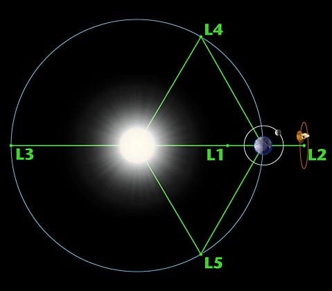
Demonstration of the Earth-Sun Lagrange points, including the WMAP location. Image courtesy NASA.
At its core, WMAP is a satellite with two 1.4m telescopes built into it, pointing 141º away from each other. The satellite is located at one of the Earth-Sun Lagrange points, meaning that the net gravitational force from the Sun + Earth is exactly equal to the centripetal force required to keep an object in a stable orbit at that point. Over the course of one orbit around the Sun, then, WMAP covers the entire sky.
The telescopes observe in five frequencies, between 23 and 94 GHz, to allow separation of emissions from within the Milky Way, which tend to be WHAT. The telescopes each feed into a differential radiometer, which measures the difference in the power (~temperature) in the same frequency between the two pointing directions. Thus it is the anisotropy that is directly measured, as opposed to any direct temperature.
Calculated quantities
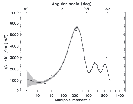
WMAP-1 power spectrum. Image from Hinshaw+2005.
1. Angular Power Spectrum – Martin White, visiting Yale a couple months ago, joked that if you give a physicist a data set, their first instinct is to take its power spectrum. In this case, that means plotting the temperature difference between points at different distances from each other. By convention, the plot shows multipole l on the x-axis instead of the angular separation, which is its reciprocal. Larger multipoles thus correspond to lower separations on the sky. Since this plot from the original paper in 2005, the error bars have grown much smaller. The most recent release, WMAP9, tests various physical models against the observed spectrum. If, as expected, this spectrum is perfectly Gaussian, then it is a complete description of the CMB anisotropy.
2. Non-Gaussianities in the CMB Anisotropy – Converse to that last point, any detected deviations from a Gaussian power spectrum suggest modifications to the standard model of cosmology.
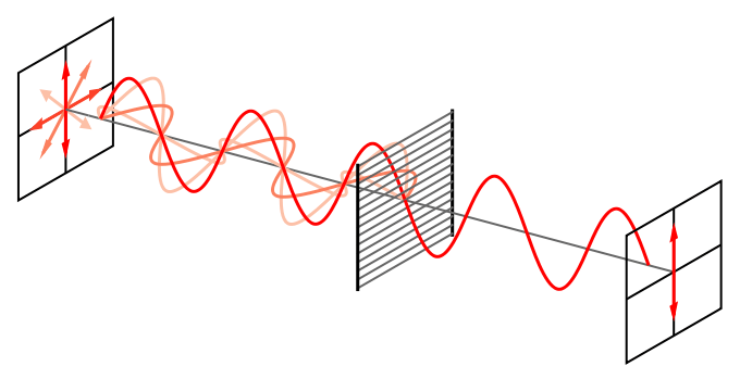
One of the fields (E or B) of unpolarized light. Image from Wikimedia Commons.
3. Polarization in the CMB – Patterns in the polarization of individual photons. You may remember that light is really electric and magnetic waves oscillating perpendicular to each other and to the direction of propagation of the light wave. But there is an entire plane perpendicular to that direction, and technically the E and B fields could be oscillating in any direction, so long as they remained perpendicular to each other. Make sense? The figure to the left should help visualize this.
Remember when Planck claimed detection of B-mode polarization in the CMB? This would have looked like the figure to the right and must not to be confused with the B-fields mentioned above. It would have been a smoking gun, as some of my macho colleagues like to say, for inflationary models of cosmology. These in turn are very popular, amongst other reasons because they naturally explain the observed flatness and uniformity of our Universe. There was this heart-warming video of Alan Guth reacting to news of the ‘discovery’ being delivered to his home. And then it turned out that polarization signal could entirely be explained by dust within the Milky Way.